引力波天文II：探测响应与灵敏度

引力波天文系列文章将介绍引力波能观测到什么，如何观测，以及基本的数据分析方法。侧重于引力波的空间探测和分析，但核心的测量原理、仪器响应以及数据分析方法基本都是通用的。

• 研究目标：波源概述(基本波源及频谱划分)
• 探测技术：响应与灵敏度、空间探测技术
• 数据分析：数据分析方法、数据分析实践

本文介绍通过激光干涉探测引力信号的基本原理，具体关注探测器对信号的响应函数以及灵敏度曲线。

基本探测原理

长波近似结论

TT transverse-traceless.

$$h(t, \vec{r}) = h_{\vec{r}=0}(t-\hat{k}\cdot \vec{r}/c) = \int \tilde{h}(f) e^{i2 \pi f(t-\hat{k}\cdot\frac{\vec{r}}{c})}$$

当$L \ll \lambda/2\pi, f \ll \frac{c}{2 \pi L}$，假设探测器位于坐标原点，有$2 \pi f \hat{k}\cdot\frac{\vec{r}}{c} \ll 1$，从而$h(t, \vec{r})$可近似简单替换为$h(t)$，忽略同一时刻探测器不同位置的信号差异，即引力波的传播效应，被称为长波近似。但光子传播过程，不同时刻的引力波信号差异仍需要考虑。

下面考虑激光沿干涉臂传播过程中受到的影响，为便于推导这里先关注单个频率成分：

$$\Delta t = \frac{1}{2c}\int_{s=0}^{L} h(s) d s= \frac{1}{2c}\int_{s=0}^{L} \tilde{h}(f) e^{i\omega t} ds$$

其中，$\vec{r}$ 和 $t$对参量$s$ 的依赖关系由激光传播决定：

$$t(s) = t|_{\vec{r}_1} + s/c = t|_{\vec{r}_2} - L/c + s/c$$

这里$\vec{r_1}, \vec{r_2}$分别为激光发射端与接收端，$\hat{x}$由激光发射端指向接收端，$t|_{\vec{r}_1}, t|_{\vec{r}_2}$ 分别为激光发射和接收时刻。注意，上式中只出现了$\hat{x}$而没有$\hat{k}$，因为上述关系完全由激光传播决定，而与引力波无关，激光是沿$\hat{x}$传播。

$$\begin{aligned} \Delta t &= \frac{1}{2c} ~\tilde{h}(f) \int_{s=0}^{L} e^{i\omega (t|_{\vec{r}_1} + \frac{s}{c})} ds\\ &= \frac{1}{2c} ~\tilde{h}(f)~ e^{i\omega t|_{\vec{r}_1}} \int_{s=0}^{L} e^{i\omega \frac{s}{c}} ds\\ &= \frac{1}{2c} ~\tilde{h}(f)~ e^{i\omega t|_{\vec{r}_1}} {\small \frac{c}{i\omega} } e^{i\omega \frac{s}{c}}\Big|_0^L\\ &= \frac{1}{2} ~\tilde{h}(f)~ e^{i\omega t|_{\vec{r}_1}} \small \frac{1}{i\omega} \left[e^{i\omega \frac{L}{c}}-1\right]\\ &= \frac{1}{2} ~\tilde{h}(f)~ e^{i\omega t|_{\vec{r}_1} } e^{i\omega \frac{2L}{c}} ~ \small \frac{2\sin\left[\omega \frac{L}{2c}\right] }{\omega}\\ &= \tilde{h}(f)~ e^{i\omega (t|_{\vec{r}_1} + \frac{L}{2c}) } ~{\small \frac{L}{2c}} ~ {\rm sinc}\left[\omega {\textstyle \frac{L}{2c}}\right]\\ \end{aligned}$$

这里$t|_{\vec{r}_1} + \frac{L}{2c}$ 对应激光传播到干涉臂中间的时间。因此对于单频引力波，单向传播的激光受到的总影响正比于干涉臂中间时的应变强度乘以${\rm sinc}$项，高频信号受到压制。${\rm sinc}$项傅里叶逆变换为$\rm rect$函数，乘积变卷积。

$$\begin{aligned} \Delta t (t|_{\vec{r}_1}) &= \frac{1}{2} h(t|_{\vec{r}_1} + {\textstyle \frac{L}{2c}}) * {\rm rect}\small \left(\frac{c}{L} t|_{\vec{r}_1} \right) \end{aligned}$$

引力波信号与矩形窗卷积，相当于信号的滑动平均，窗口宽度为$\frac{L}{c}$，测量效应为引力波信号的平均。

代入$t|_{\vec{r}_1} = t|_{\vec{r}_2} - \frac{L}{c}$，用接收端的时间和位矢表示有：

$$\begin{aligned} \Delta t &= \tilde{h}(f) e^{i\omega (t|_{\vec{r}_2} - \frac{L}{2c})} ~ {\small \frac{L}{2c}} ~ {\rm sinc}\left[\omega {\textstyle \frac{L}{2c}}\right] \end{aligned}$$

除了时间(相位)变化，对引力波效应的另一个常用描述是分数多普勒频移$\frac{\Delta \nu}{\nu} = \frac{\nu_{\rm recv} - \nu_{\rm emit}}{\nu_{\rm emit}}$。PTA相关文献中通常记为符号$z$，而在空间引力波探测中更常用$y$表示。根据相位关系：

$$\phi_{\rm recv} = \phi_{\rm emit} + 2 \pi \nu_{\rm emit}\frac{L}{c} + 2 \pi \nu_{\rm emit}\Delta t$$

求导可得$\frac{\Delta \nu}{\nu} = \dot{\Delta t} = i\omega \Delta t$，从而：

$$\begin{aligned} \Delta t &= \frac{1}{2}~\tilde{h}(f)~ e^{i\omega t|_{\vec{r}_1}} \small \frac{1}{i\omega } \left[e^{i\omega\frac{L}{c}}-1\right]\\ \frac{\Delta \nu}{\nu} & = \frac{1}{2}~\tilde{h}(f)~ e^{i\omega t|_{\vec{r}_1}} \left[e^{i\omega\frac{L}{c}}-1\right]\\ & = \frac{1}{2} \left[\tilde{h}(f)~e^{i\omega t|_{\vec{r}_2} } - \tilde{h}(f)~e^{i\omega t|_{\vec{r}_1}} \right] \end{aligned}$$

傅里叶逆变换

$$\begin{aligned} y(t) &= \frac{1}{2} \left[ h(t|_{\vec{r}_2}) - h(t|_{\vec{r}_1}) \right] \end{aligned}$$

这里$\vec{r_1}, \vec{r_2}$分别对应激光发射端与接收端，$t|_{\vec{r}_1}, t|_{\vec{r}_2}$ 则对应激光的发射和接受时间。即，引力波导致的多普勒频移仅由接收时刻(接收端)与发射时刻(发射端)的应变强度之差决定！

除了这里通过对光子路径积分获得距离变化，对应相位改变，求导可得到频率变化。还可以直接推导频率影响，之后积分得到相位改变。
高阶速度项的影响可忽略(Cornish & Rubbo 2003)

最后，对于单臂往返，发射与接收端重合，将最终接收时间$t_{\rm recv}$简记为$t$，考虑往返的总效应，有：

$$\begin{aligned} \Delta t &= \frac{1}{2}~\tilde{h}(f)~ e^{i\omega (t - \frac{L}{c}) } \small \frac{1}{i\omega} \left[e^{i\omega \frac{L}{c}} - 1\right] + \frac{1}{2}~\tilde{h}(f)~ e^{i\omega (t - \frac{2L}{c})} \small \frac{1}{i\omega } \left[e^{i\omega \frac{L}{c}}-1\right]\\ &= \frac{1}{2}~\tilde{h}(f)~ e^{i\omega t } \small \frac{1}{i\omega} \left[ 1 - e^{-i\omega \frac{2L}{c}} \right]\\ &= \frac{1}{2}~\tilde{h}(f)~ e^{i\omega (t -\frac{L}{c}) } {\textstyle \frac{2L}{c}} {\rm sinc}\left[\omega {\textstyle \frac{L}{c}}\right] \end{aligned}$$

$$\begin{aligned} \tilde{y}(f) &= \frac{1}{2}~\tilde{h}(f)~ \left[1- e^{-i\omega\frac{2L}{c}} \right] e^{i\omega t}\\ &= \frac{1}{2} ~\tilde{h}(f)~ e^{i\omega t} ~ 2i~ \sin\left({\textstyle \omega\frac{L}{c} }\right)~e^{-i\omega\frac{L}{c}} \\ \end{aligned}$$

$$\begin{aligned} y(t) = \frac{1}{2} \left[ h(t) - h(t-{\textstyle \frac{2L}{c} }) \right]\\ \end{aligned}$$

$$\boxed{\begin{aligned} \Delta t &= \frac{1}{2}~\tilde{h}(f)~ e^{i\omega (t - \frac{L}{c})} {\textstyle \frac{2L}{c} } {\rm sinc}\left[\omega {\textstyle \frac{L}{c}}\right] \end{aligned}}$$

如果将上述时间变化量转换为对应的无量纲应变响应，有：

$$\begin{aligned} s(f, t, \hat{x}, \hat{k}, \vec{r}_1) &\equiv {\small \frac{\Delta L}{L}} = \frac{c \Delta t/2}{L} = \frac{1}{2}~\tilde{h}(f)~ e^{i 2\pi f (t - \frac{L}{c})} {\rm sinc}\left[\omega {\textstyle \frac{L}{c}}\right] \end{aligned}$$

注意，这里$\Delta L = c \Delta t/2$，因为$\Delta t$为往返时长差，因此光程差对应于2倍的臂长差。
$s(f,t)$就是激光臂对单个频率成分 $\tilde{h}(f)e^{i\omega t}$ 的响应。可以看到响应是线性的，即$s \propto \tilde{h}(f)e^{i\omega t}$，因此总的引力波响应就是所有频率分量贡献的线性叠加，即对频率积分。用$\mathscr{D}$表示探测器响应：

$$\begin{aligned} s(t) &= \mathscr{D}\left(h(t)\right) = \mathscr{D}\left(\int \tilde{h}(f)e^{i 2\pi f t} df\right)\\ &= \int \mathscr{D}\left(\tilde{h}(f)e^{i 2\pi f t}\right) df = \int s(f, t) df\\ &= \int df ~ \frac{1}{2}~\tilde{h}(f)~e^{i 2\pi f t} ~\mathcal{T}(f, \hat{k} \cdot \hat{x})\\ &= \int \left[ \frac{1}{2}~\tilde{h}(f)~~\mathcal{T}(f, \hat{k} \cdot \hat{x}) \cdot \hat{x})\right] ~e^{i 2\pi f t} df \end{aligned}$$

$$\begin{aligned} \tilde{s}(f) &= \mathcal{F}\left\{s(t)\right\} = \frac{1}{2}~\tilde{h}(f)~ e^{-i \omega\frac{L}{c}} {\rm sinc}\left[\omega {\textstyle \frac{L}{c}}\right] \end{aligned}$$

至此还只是单臂往返，其中$h(t)$是引力波信号在探测臂方向的投影，依赖其具体指向，张量形式为$\hat{x}^i\hat{x}^j h_{ij}(t)$。从而对于双臂干涉

$$\boxed{\begin{aligned} \tilde{y}(f) &= \frac{1}{2} \left[1- e^{-i\omega\frac{2L}{c}} \right] \left[\hat{x}^i \hat{x}^j - \hat{y}^i \hat{y}^j \right] \tilde{h}_{ij}(f)\\ &= \frac{1}{2} ~2i~ e^{-i\omega\frac{L}{c}}~\sin\left({\textstyle \omega\frac{L}{c} }\right) \left[\hat{x}^i \hat{x}^j - \hat{y}^i \hat{y}^j \right] \tilde{h}_{ij}(f) \end{aligned}}$$

$$\boxed{\begin{aligned} \tilde{s}(f) &= \frac{1}{2} ~{\small \frac{1}{i\omega}~ \frac{1}{2L/c}}~ \left[1- e^{-i\omega\frac{2L}{c}} \right] \left[\hat{x}^i \hat{x}^j - \hat{y}^i \hat{y}^j \right] \tilde{h}_{ij}(f)\\ &= \frac{1}{2} ~ e^{-i \omega\frac{L}{c}}~ {\rm sinc}\left[\omega {\textstyle \frac{L}{c}}\right] \left[\hat{x}^i \hat{x}^j - \hat{y}^i \hat{y}^j \right] \tilde{h}_{ij}(f) \end{aligned}}$$

对比两者，区别在于$\sin$变为$\rm sinc$，没有虚数单位$\rm i$，同时因为$\Delta L/2L$消去了原本的2倍。
如果进一步做长波近似，取$f \rightarrow 0$，则可得到更常见的长波近似结果：

$$\boxed{\begin{aligned} \tilde{y}(f) &= {\small i \frac{\omega L}{c} } \left[\hat{x}^i \hat{x}^j - \hat{y}^i \hat{y}^j \right] \tilde{h}_{ij}(f)\\ \tilde{s}(f) &= \frac{1}{2} ~\left[\hat{x}^i \hat{x}^j - \hat{y}^i \hat{y}^j \right] \tilde{h}_{ij}(f) \end{aligned}}$$

---

引力波对时空的扰动会影响光束经过测底线上两点的时间间隔，进而反映在相位测量上，这是现代引力波测量的基本原理。在平直时空中任取两点，连线方向设为$x$轴，对应空间坐标分别为$(0,0,0)$和$(L,0,0)$。只考虑$x$方向($dy=dz=0$)，假设引力波引入的时空微扰在$x$方向的投影为$h(t)$，所对应的线元可表示为：

$$ds^2 = g_{\mu\nu} dx^\mu dx^\nu = -c^2dt^2 + [1+h(t)]dx^2$$

$$ds^2 = g_{\mu\nu} dx^\mu dx^\nu = -c^2dt^2 + [1+h_+(t)]dx^2 + [1+h_\times(t)]dx^2 + dz^2$$

这里暂时只考虑$x$方向的引力波观测效应，并暂时将$h_+(t)$简记为$h(t)$。光线沿零测地线(null geodesic)移动$ds^2 = 0$，从而对于沿$x$方向传播的光$c dt = \sqrt{1 + h_+(t)}dx$。这就是用光进行(干涉)测量的基本原理，即对光而言时空距离的改变会反映在坐标时间中，并最终通过相位观测记录。由发射点到接收点积分：

$$c(t_{\rm recv} -t_{\rm emit}) = \int_{t_{\rm emit}}^{t_{\rm recv}} c dt = \int_0^L \sqrt{1 + h[t(x)]}dx \approx \int_0^L \left\{1 +\frac{1}{2}h[t(x)]\right\}dx$$

这里利用$h(t) \ll 1$做了一阶近似展开。最终光信号到达接收点时间为：

$$t_{\rm recv} \approx t_{\rm emit} + \frac{L}{c} + \frac{1}{2c} \int_0^L h[t(x)] dx$$

最后一项为引力波引入的修正，但积分反过来又依赖自身$t(x)$，通常需迭代。一阶近似取$t(x) = t_{\rm emit} + \frac{x}{c}$，接收端对应时间为：

$$t_{\rm recv} \approx t_{\rm emit} + \frac{L}{c} + \frac{1}{2c} \int_0^L h\left(t_{\rm emit} + \frac{x}{c}\right) dx = t_{\rm emit} + \frac{L}{c} + \frac{1}{2} \int_{t_{\rm emit}}^{t_{\rm emit} + \frac{L}{c}} h(t) dt$$

最后一项为引力波引入的一阶修正，进一步迭代所引入的高阶修正量为$o(h^2)$量级，这里暂时忽略。最终，引力波效应为：

$$\boxed{\begin{aligned} \Delta t &= t - t_{\rm emit} - \frac{L}{c} = \frac{1}{2} \int_{t-\frac{L}{c}}^{t} h(\tau) d\tau\\ \Delta L &= c\Delta t =\frac{c}{2} \int_{t-\frac{L}{c}}^{t} h(\tau) d\tau \end{aligned}}$$

考虑到相位测量是在接收端进行，这里调整了积分限，并将$t_{\rm recv}$简记为$t$，并不影响结果。最终相位测量：

$$\varphi_{\rm recv} \approx \varphi_{\rm emit} + 2\pi\nu_0\frac{L}{c} + 2\pi\nu_0\Delta t$$

其中$2\pi \nu_0 \Delta t$为引力波引入的相位偏移，$\nu_0$为激光发射频率。通过激光干涉技术，可以对该相位偏移做出精确测量，这是现代引力波测量的核心。地基引力波探测处于长波极限，$L \ll \lambda$，波长覆盖整个探测器，引力波振幅在两点间变化不大，积分内的$h(t)$可近似为常数，从而$\Delta L = \frac{1}{2} L h(t) \propto h(t)$。

对于单频信号，取$h(t) = h_0 e^{-i\omega t}$，带入前面的公式有：

$$\begin{aligned} \Delta t &= \frac{1}{2} \int_{t-\frac{L}{c}}^{t} h_0 e^{-i\omega \tau} d\tau = \frac{h_0}{2} \frac{1}{-i\omega} e^{-i\omega \tau}\Big|_{t-\frac{L}{c}}^{t} \\ &= \frac{h_0}{2} \frac{1}{-i\omega} e^{-i\omega t} \left[1 - e^{i\omega \frac{L}{c}}\right]\\ & = h_0 e^{-i\omega t} e^{i\omega \frac{L}{2c}} \frac{\sin(\omega \frac{L}{2c})}{\omega} \end{aligned}$$

简单整理有：

$$\boxed{\Delta t = {\small \frac{L}{2c}} ~ h(t-{\textstyle \frac{L}{2c}}) ~ {\rm sinc}(\omega {\textstyle \frac{L}{2c}})}$$

这里${\rm sinc}(x) = \frac{\sin x}{x}$，在长波极限下$L \ll \lambda, \omega \frac{L}{2c} \ll \pi$，${\rm sinc}(\omega \frac{L}{2c}) \sim 1$。而随着引力波频率增加，$\omega \frac{L}{2c} \gtrsim \pi$，引力波信号将比显著抑制。注意，这里测量信号依赖$h(t- {\textstyle \frac{L}{2c}})$，如果是沿$x$方向往返，$L \rightarrow 2L$，则对应于在远端反射时刻的信号强度。

另一个方面，对前面公式两边求导有：

$$2\pi\nu(t) \approx 2\pi\nu_0 + 2\pi\nu_0\dot{\Delta t} = 2\pi\nu_0 + 2\pi\nu_0 \frac{1}{2} \Big[h(t) - h(t - {\textstyle \frac{L}{c}})\Big]$$

这里利用了变限积分的导数，假设激光发射频率稳定为$\nu_0$，并定义瞬时频率$\nu(t) = \frac{\dot{\varphi}(t)}{2\pi}$。简单整理有：

$$\boxed{\frac{\nu(t)-\nu_0}{\nu_0} \approx \frac{1}{2} \Big[h(t) - h(t - {\textstyle \frac{L}{c}})\Big]}$$

即接收到的激光瞬时频率相对发射端基准频率的相对偏移正比于引力波在两点的振幅差。直观理解，引力波的波峰或波谷的到达时间受到引力波调制，最终的接收频率也将随之发生变化。长波极限下，$h(t)$在光传播过程中近似常数，$\frac{\nu(t)-\nu_0}{\nu_0} \approx 0$，因此地基引力波探测无需考虑频率偏移，但对于空间引力波探测，激光频率的相对偏移是经常讨论的物理量，后面会具体展开。值得注意的，这里激光的频率偏移仅依赖引力波在两端点时刻的引力波振幅，而与激光传播过程中的引力波演化无关(不限制$h(t)$的形式)！

激光干涉测量

https://en.wikipedia.org/wiki/Interferometry
https://en.wikipedia.org/wiki/Sagnac_effect
https://en.wikipedia.org/wiki/Common-path_interferometer#Zero-area_Sagnac
后面会提到，激光的频率噪声远高于引力波测量所需精度，因此上述单臂单向响应在实际的激光测量中并不现实，需要等臂干涉抑制激光频率噪声。而反过来说，如果计时精度足够，则无需干涉，这正是脉冲星计时用于引力波测量的原理。注意，脉冲星观测中实现计时所依靠的并非射电辐射本身的频率精度，而是射电脉冲间隔(脉冲到达时间)精度。因此，对脉冲星计时测量而言，多普勒频移是脉冲间隔的频移，而非电磁波本身频移（虽然两者受引力影响相同？？），后者对应多普勒追踪(Doppler tracking)测量，属于另一种引力波测量方法。最后，脉冲计时测量随机背景时，需要在不同脉冲星测量间进行互相关，注意区分相关分析与干涉测量，干涉仪测量背景引力波时同样需要不同探测器间进行相关分析。

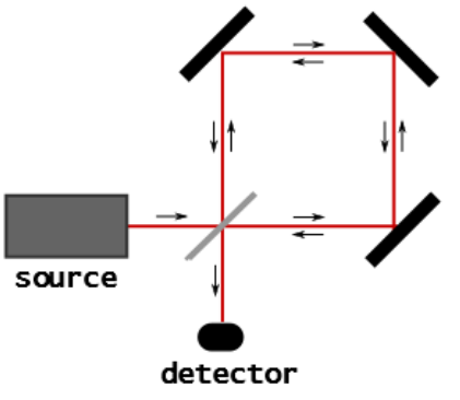
对于引力波测量而言，两种常见的激光干涉主要有迈克尔逊干涉(Michelson)和萨格纳克干涉(Sagnac)。如下图所示，两者的主要区别在于光线的传播路径：前者经过分光的两束光线走不同路径进行干涉，而后者则是经过相同路径进行干涉。

迈克尔逊干涉更为知名，当前运行的aLIGO, Adv-Virgo等都属于迈克尔逊干涉。
早在狭义相对论提出(1905)之前，Michelson为了检验以太理论，于1881年首次构想并实施了激光干涉测量，并在之后通过改进的迈克尔逊-莫雷实验(1887)否定了“以太”理论，而被载入史册，直接推动了洛伦兹变换的提出及狭义相对论的发展。迈克尔逊1886年就提出过激光干涉的萨格纳克构型，随后又被萨格纳克重新提出(Sagnac 1913)，而广义相对论的提出则要到更晚的1915年。

萨格纳克效应用于激光或光纤陀螺仪

迈克尔逊干涉实验是非常著名的相对论检验实验，但萨格纳克效应

而将萨克纳克干涉用于引力波测量的想法很早就有人提出(R. W. P. Drever 1983, R.Weiss 1987, Sun et al. 1996)，
为此人们提出了零面积的萨格纳克干涉与LIGO的构型非常接近，只是在分光镜附近增加了一个反射镜，使得两束光经相同路径后再干涉。
在讨论下一代引力波探测器时，除了延续迈克尔逊干涉思路的CE、ET，基于萨格纳克干涉的设想同样被不断提及。

萨格纳（Sagnac）原理：也称萨氏效应（相位差正比于输入角速率）。该原理适用于光纤角速率陀螺；激光角速率陀螺等。Sagnac法国物理学家（1869年～1926年），居里夫妇的朋友。1913年发明萨氏效应。

As noted above, Sagnac interferometers are, to first order, insensitive to any static or low-frequency displacement of their optical components, nor are the fringes affected by minor frequency variation in the lasers or birefringence.
This variant of the Sagnac interferometer is hence insensitive to rotation or low frequency drift of its optical components,

insensitive to rotations while remaining sensitive to time-dependent displacement in the two arms.
Sun et al. have investigated the possibility of detecting a broad-band GW detector with a zeroarea Sagnac interferometer.

外差干涉测量

两个频率接近的电磁波信号相干叠加，其电场强度可表示为(这里假设两个信号偏振方向相同)：

$$E_s\cos(\omega_s t + \phi) + E_{\rm LO}\cos(\omega_{\rm LO} t)$$

在探测器进行探测时，光电感应器的响应信号与光强而非场强成正比(非线性响应)，而光强

$$\begin{aligned} I \propto ~&~ [E_s\cos(\omega_s t + \phi) + E_{\rm LO}\cos(\omega_{\rm LO} t)]^2\\ =~&~ E_s^2\cos^2(\omega_s t + \phi) + E_{\rm LO}^2\cos^2(\omega_{\rm LO} t) + 2E_sE_{\rm LO}\cos(\omega_s t + \phi)\cos(\omega_{\rm LO} t)\\ =~&~ \frac{1}{2}E_s^2[1+\cos 2(\omega_s t + \phi)] + \frac{1}{2}E_{\rm LO}^2[1+\cos(2\omega_{\rm LO} t)]\\ ~&~ + E_sE_{\rm LO}\big\{cos[(\omega_s-\omega_{\rm OL}) t + \phi] + \cos[(\omega_s+\omega_{\rm OL}) t + \phi]\big\} \end{aligned}$$

探测器只能探测到信号在响应时间内的积分(平均强度)，考虑到光电感应器响应时间≫信号本身周期，上式中的高频项积分响应为0，从而最终的响应

$$\propto \frac{1}{2}(E_s^2+E_{\rm LO}^2) + E_sE_{\rm LO}\cos[(\omega_s-\omega_{\rm OL}) t + \phi]$$

也可以解释为，通过低通滤波移除了所有高频信号。在目标信号与参考输入频率差值足够小时，差频(拍频)项$\omega_s-\omega_{\rm OL}$将得以保留。而当$\omega_s$与$\omega_{\rm LO}$相等，系统响应

$$\propto \frac{1}{2}(E_s^2+E_{\rm LO}^2) + E_sE_{\rm LO}\cos \phi$$

外差干涉与零差干涉

• 探测器实际响应的是$E_sE_{\rm LO}$项，相比信号本身($E_s^2$)，通过增强$E_{\rm LO}$可实现弱信号的增益放大。
• 相位差值信息得到了完美保留，可以实现相位的线性响应
• 拍频降低频率，可以实现相位差值或频率偏移的精确测量

拍频越低，测量精度越高，但为什么不能太低？
外差干涉需要细致的频段规划(frequency plan)，同时通过自适应技术保持六路拍频尽可能低，但又不为零(或跨越零)。而为了确保卫星漂移的多普勒效应是频率偏移的唯一来源，所有激光的频率需要相互锁定，并最终与稳定的参考基准保持锁定。

同时由于卫星运动的多普勒效应，在MHz量级，为了拍频不跨越零，

激光功率不稳定性在-5Hz~5Hz内占据主导，因此拍频信号需要避开该频段，即频率下限为5Hz。

下限为6MHz，
通过合适的锁频算法，拍频够可以保持在7~23MHz

考虑到为本身多普勒效应在MHz量级，为保证拍频不跨越零，也需要至少为MHz量级，在5~25MHz之间波动

仪器响应函数

$$\Delta t =$$

正交性

$$\int \frac{d\hat{k}}{4\pi} F_+F_\times = 0$$

平均响应

$$\int \frac{d\hat{k}}{4\pi} F_+ \neq \int \frac{d\hat{k}}{4\pi} F_\times; ~~~~ \int \frac{d\psi}{2\pi} F_+ = \int \frac{d\psi}{2\pi} F_\times$$

$$\int \frac{d\psi}{2\pi} \int \frac{d\hat{k}}{4\pi} F_+ = \int \frac{d\psi}{2\pi} \int \frac{d\hat{k}}{4\pi} F_\times$$

对给定的引力波信号$h_{ij}$，时空伸缩模式是确定的，有确定的特殊标架方向。
对于单个探测器而言，$\psi$是冗余，改变张量极化基矢，最终响应旋转不变，也就是无法测偏振？

天线模式函数

探测器坐标系、日心坐标系、潮汐效应、相对论效应
需要对轨道进行数值积分，以达到所需精度

探测器对于信号的响应依赖空间方位，被称为天线响应模式(antenna response pattern)或简单的天线模式(antenna pattern)，也可称为天线的指向性函数(antenna directivity)或天线波束(antenna beam pattern)，后者在射电领域更常见。对于引力波探测而言，天线模式具体依赖天线构型和引力波的方位及偏振。

广义相对论框架下，采用横向无迹(TT)规范，引力波为横波且只有两种偏振模式，在垂直引力波传播平面内

$$\begin{aligned} \bm{h} = \begin{pmatrix} h_{+} & h_{\times} \\ h_{\times} & -h_{+} \end{pmatrix} = h_{+} \begin{pmatrix} 1 & 0 \\ 0 & -1 \end{pmatrix} + h_{\times}\begin{pmatrix} 0 & 1\\ 1 & 0 \end{pmatrix} = h_{+} \bm{e}^{+} + h_{\times}\bm{e}^{\times} \end{aligned}$$

其中$\bm{e}^{+}, \bm{e}^{\times}$代表引力波的两种张量偏振模式，$h_{+}, h_{\times}$为对应的强度。在广义相对论之外，引力波还可以有横向的呼吸模式、沿传播方向的纵向模式(纵波)以及横纵交叉的矢量模式。直角坐标系下，引力波的张量模式可通过矢量外积(张量积)描述：

$$\begin{aligned} \bm{e}^{+} &= \hat{u} \otimes \hat{u} - \hat{v}\otimes \hat{v}\\ \bm{e}^{\times} &= \hat{u}\otimes \hat{v} + \hat{v}\otimes \hat{u}\\ \bm{e}^{\circ} &= \hat{u} \otimes \hat{u} + \hat{v}\otimes \hat{v}\\ \bm{e}^{l} &= \hat{k}\otimes \hat{k} \\ \bm{e}^{x} &= \hat{u} \otimes \hat{k} - \hat{k}\otimes \hat{u}\\ \bm{e}^{y} &= \hat{v}\otimes \hat{k} + \hat{k}\otimes \hat{v} \end{aligned}$$

这里$\hat{u}, \hat{v}, \hat{k}$为直角坐标系基矢，其中$\hat{k}$为引力波传播方向，$\hat{u}, \hat{v}$沿$+$模式伸缩方向，$\times$模式相对旋转45°，此时引力波偏振度为0。下面暂不考虑张量模式之外的偏振。
在垂直传播方向的平面内取$\hat{p}, \hat{q}$，相对$\hat{u}, \hat{v}$顺时针旋转$\psi$角，或者说引力波$+$模式主轴相对参考系$\hat{p}, \hat{q}$逆时针旋转$\psi$角则：

$$\begin{aligned} \bm{h} &= \bar{h}_{+} \bm{\epsilon}^{+} + \bar{h}_{\times}\bm{\epsilon}^{\times}\\ \bm{\epsilon}^{+} &= \hat{p}\otimes \hat{p} - \hat{q}\otimes \hat{q}\\ \bm{\epsilon}^{\times} &= \hat{p}\otimes \hat{q} + \hat{q}\otimes \hat{p} \end{aligned}$$

$$\begin{aligned} \begin{pmatrix} \hat{p} \\ \hat{q} \end{pmatrix} = \mathcal{R}_{\psi} \begin{pmatrix} \hat{u} \\ \hat{v} \end{pmatrix} ; ~~~~~ \mathcal{R}_{\psi} = \begin{pmatrix} \cos \psi & -\sin \psi \\ \sin \psi & \cos \psi \end{pmatrix} \end{aligned}$$

$$\begin{aligned} \begin{pmatrix} \hat{p} \\ \hat{q} \end{pmatrix}\otimes \begin{pmatrix} \hat{p} \\ \hat{q} \end{pmatrix} = \left[\mathcal{R}_{\psi} \begin{pmatrix} \hat{u} \\ \hat{v} \end{pmatrix}\right] \otimes \left[\mathcal{R}_{\psi} \begin{pmatrix} \hat{u} \\ \hat{v} \end{pmatrix}\right] = \mathcal{R}_{\psi} \left[\begin{pmatrix} \hat{u} \\ \hat{v} \end{pmatrix} \otimes \begin{pmatrix} \hat{u} \\ \hat{v} \end{pmatrix}\right] \mathcal{R}^T_{\psi} \end{aligned}$$

$$\begin{aligned} \mathcal{R}_{\psi} \begin{pmatrix} h_+ & h_\times\\ h_\times & - h_+ \end{pmatrix} \mathcal{R}^T_{\psi} = \mathcal{R}_{\psi}\mathcal{R}_{\psi} \begin{pmatrix} h_+ & h_\times\\ h_\times & - h_+ \end{pmatrix} = \mathcal{R}_{2\psi} \begin{pmatrix} h_+ & h_\times\\ h_\times & - h_+ \end{pmatrix} \end{aligned}$$

这个对普通矩阵不成立，是这种特殊情况下的结果？

$$??\begin{aligned} \begin{pmatrix} \bar{h}_{+} \\ \bar{h}_{\times} \end{pmatrix} = \mathcal{R}_{2\psi} \begin{pmatrix} h_{+} \\ h_{\times} \end{pmatrix}, ~ \begin{pmatrix} \bm{\epsilon}^{+} \\ \bm{\epsilon}^{\times} \end{pmatrix} = \mathcal{R}_{2\psi} \begin{pmatrix} \bm{e}^{+} \\ \bm{e}^{\times} \end{pmatrix} \end{aligned}??$$

这里$\psi$就是引力波在 $\hat{p}, \hat{q}$ 参考系下的偏振角。注意，引力波是四极辐射，因此实际旋转矩阵角度为$2\psi$，旋转$\frac{\pi}{4}$两种偏振模式互换(伸缩反相)，旋转$\frac{\pi}{2}$回到初始偏振(伸缩反相)。

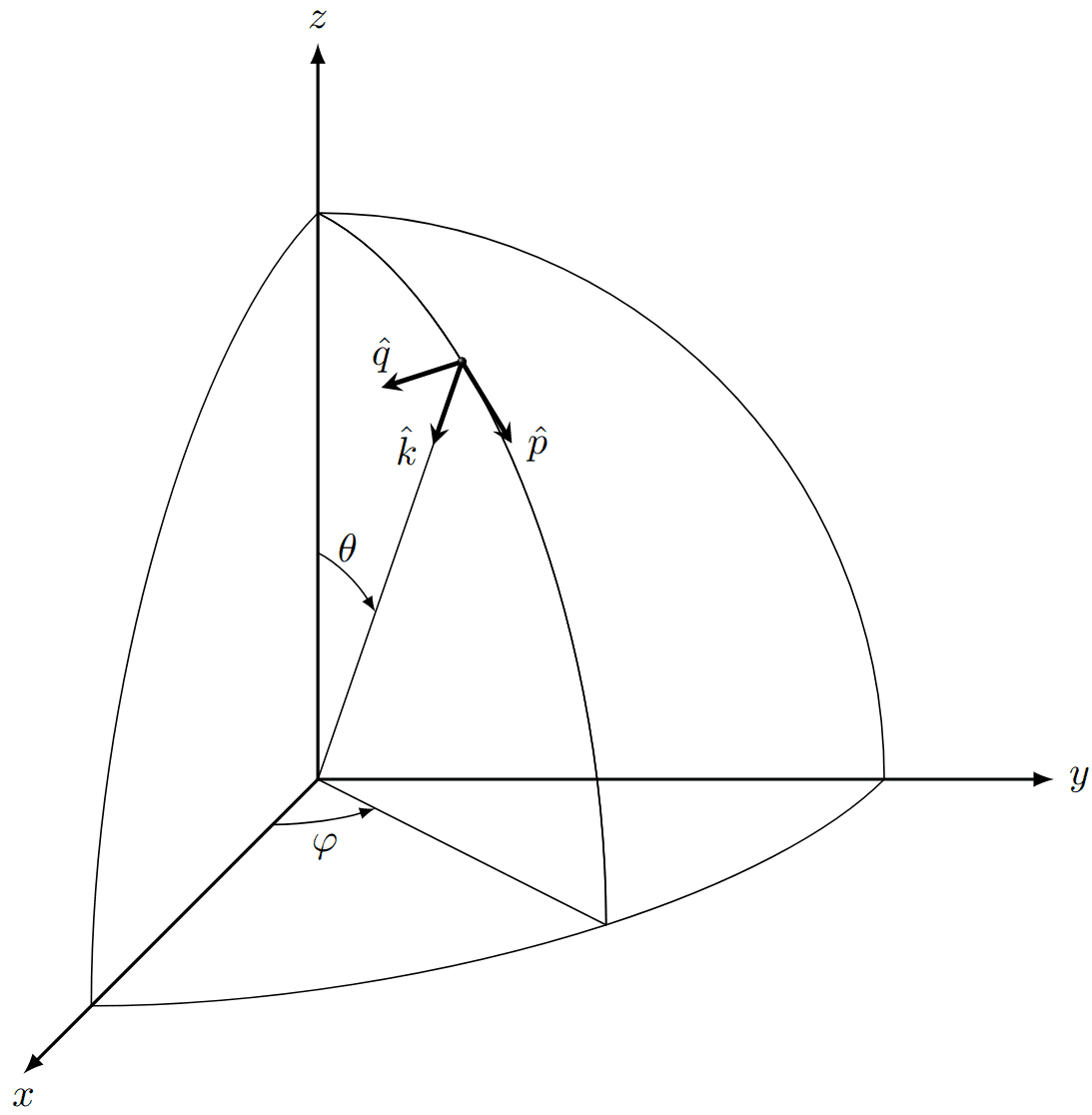
下面讨论探测器对引力波的响应，如下图所示，考虑直角的迈克尔逊干涉仪，沿引力波探测臂建立坐标系，引力波沿$\hat{k}$方向到达探测器，对应方位角$(\theta, \varphi)$。这里引力波由$x,y$平面下向上传播，由上至下的传播对应$\theta >\pi/2$。

We denote by $\theta, \varphi$ the angles that define the propagation direction $\hat{k}$ of the GW from the source to us, so the polar angles of the source, as seen from the Earth, are $\theta_s = \pi - \theta$ and $\varphi_s = \pi + \varphi$.

首先考虑单臂情况，探测信号对应应变张量在探测臂方向的投影，对$x$轴方向的探测臂：

$$\boxed{h_{xx} = \frac{1}{2}~\hat{x}\otimes\hat{x} : \bm{h} = \frac{1}{2}~\hat{x}\cdot \bm{h} \cdot \hat{x}}$$

其中$\hat{x}\otimes \hat{x}$为$x$方向上的投影算符。代入引力波应变张量：

$$\begin{aligned} h_{xx} = \frac{1}{2}~\hat{x}\otimes\hat{x} : \begin{pmatrix} \bar{h}_{+} & \bar{h}_{\times} \end{pmatrix} \begin{pmatrix} \bm{\epsilon}^{+}\\ \bm{\epsilon}^{\times} \end{pmatrix} = \frac{1}{2}\begin{pmatrix} \bar{h}_{+} & \bar{h}_{\times} \end{pmatrix} \begin{pmatrix} \hat{x}\cdot \bm{\epsilon}^{+} \cdot \hat{x}\\ \hat{x} \cdot \bm{\epsilon}^{\times} \cdot \hat{x} \end{pmatrix} \end{aligned}$$

同时，探测信号用响应函数表示有：

$$h = F^P h_P = \begin{pmatrix} h_{+} & h_{\times} \end{pmatrix} \begin{pmatrix} F^{+} \\ F^{\times} \end{pmatrix} = \begin{pmatrix} \bar{h}_{+} & \bar{h}_{\times} \end{pmatrix} \begin{pmatrix} D^{+} \\ D^{\times} \end{pmatrix}$$

其中$A$对应偏振模式，这里仅考虑广义相对论框架下的两种偏振，对比两式有：

$$\boxed{ F_{x}^P = \frac{ \hat{x}\cdot \bm{e}^P \cdot \hat{x} }{2};~~~ D_{x}^P = \frac{ \hat{x}\cdot \bm{\epsilon}^P \cdot \hat{x} }{2} }$$

$$\begin{aligned} D_{x}^{+} &= \frac{\hat{x}\cdot \bm{\epsilon}^{+} \cdot \hat{x}}{2} = \frac{(\hat{p}\cdot \hat{x})^2 - (\hat{q}\cdot \hat{x})^2}{2} \\ D_{x}^{\times} &= \frac{\hat{x} \cdot \bm{\epsilon}^{\times} \cdot \hat{x}}{2} = (\hat{p}\cdot \hat{x})(\hat{q}\cdot \hat{x}) \end{aligned}$$

根据球坐标系与直角坐标基矢关系 $\hat{\theta}\cdot\hat{x} = \cos\theta\cos\varphi, ~\hat{\varphi}\cdot\hat{x} = {\footnotesize -}\sin\varphi$ 有：

$$\hat{p}\cdot\hat{x} = \cos\theta\cos\varphi, ~~~ \hat{q}\cdot\hat{x} = \sin\varphi$$

从而：

$$\begin{aligned} D_x^{+}(\theta, \varphi) &= \frac{\cos^2\theta \cos^2\varphi - \sin^2\varphi}{2}\\ D_x^{\times}(\theta, \varphi) &= \cos\theta \cos\varphi \sin\varphi\\ \end{aligned}$$

指向函数体现了天线对不同方向上信号的相对灵敏度：引力波沿探测臂方向($\theta=\frac{1}{2}\pi, \varphi=0, \pi$)，探测器完全无响应；引力波垂直探测臂方向($\varphi=\frac{1}{2}\pi,\frac{3}{2}\pi$)时，对$+$模式响应取最大值$\frac{1}{2}$，但对$\times$模式同样无响应。疑问：当$\theta=0, \pi$，$\varphi$取值不改变引力波传播方向，但响应函数依赖$\varphi$，这点如何理解？

类似的，对$y$方向的探测器 $h_{yy}(t) = \frac{1}{2}~\hat{y}\otimes\hat{y} : \bm{h}(t)$

$$\hat{p}\cdot\hat{x} = \cos\theta\sin\varphi ; ~~~ \hat{q}\cdot\hat{y} = -\cos\varphi$$

$$\begin{aligned} D_{y}^{+} &= \frac{\hat{y}\cdot \bm{\epsilon}^{+} \cdot \hat{y}}{2} = \frac{(\hat{p}\cdot \hat{y})^2 - (\hat{q}\cdot \hat{y})^2}{2} \\ D_{y}^{\times} &= \frac{\hat{y} \cdot \bm{\epsilon}^{\times} \cdot \hat{y}}{2} = (\hat{p}\cdot \hat{y})(\hat{q}\cdot \hat{y}) \end{aligned}$$

从而：

$$\begin{aligned} D_y^{+}(\theta, \varphi) &= \frac{\cos^2\theta \sin^2\varphi {\footnotesize -} \cos^2\varphi}{2}\\ D_y^{\times}(\theta, \varphi) &= -\cos\theta \sin\varphi \cos\varphi \end{aligned}$$

对于迈克尔逊双臂干涉，总体响应为两个方向响应之差，即：

$$\begin{aligned} D^P = \frac{1}{2}\hat{l}_1\otimes\hat{l}_1 : \bm{e}^P - \frac{1}{2}\hat{l}_2\otimes\hat{l}_2 : \bm{e}^P = \frac{\hat{l}_1\otimes\hat{l}_1 - \hat{l}_2\otimes\hat{l}_2}{2} : \bm{e}^P \end{aligned}$$

注意，在这种形式本身不要求干涉臂方向 $\hat{l}_1, \hat{l}_2$ 垂直，只需要将
这里干涉臂方向矢量不用$\hat{x},\hat{y}$，用$\hat{p},\hat{q}$、$\hat{u},\hat{v}$或 $\hat{l}_1, \hat{l}_2$

对于直角的迈克尔逊双臂干涉而言，总体响应为两者之差：

$$\begin{aligned} D^P = \frac{\hat{x}\otimes\hat{x} - \hat{y}\otimes\hat{y}}{2} : \bm{e}^P \end{aligned}$$

$$\begin{aligned} D^{+}(\theta, \varphi) &= D_x^{+} - D_y^{+} = \frac{1}{2}(1+\cos^2\theta)\cos2\varphi\\ D^{\times}(\theta, \varphi) &= D_x^{\times} - D_y^{\times} = \cos\theta\sin2\varphi \end{aligned}$$

$$D_{\rm rms}(\theta, \varphi) = \sqrt{ {D^{+}}^2 + {D^{\times}}^2 } = \sqrt{\frac{1}{4}\sin^4\theta\cos^2 2\varphi + \cos^2\theta}$$

对单独的极化模式：
两种极化模式均方根响应：
垂直探测器平面时响应最强
探测器角平分线或平行探测器平面且垂直角平分线时响应最弱
立体图和天球图两个视角下理解

import numpy as np
import matplotlib.pyplot as plt
from mpl_toolkits.mplot3d import Axes3D

def plot_beam_pattern(F, theta, phi, fig, viewangle=()):
    # Convert spherical coordinates to Cartesian coordinates
    r = np.abs(F)
    x = r * np.sin(theta) * np.cos(phi)
    y = r * np.sin(theta) * np.sin(phi)
    z = r * np.cos(theta)

    # Create a 3D plot
    ax = fig.add_subplot(111, projection='3d')
    ax.view_init(10, 35) #view angle: inclination, azimuth

    # Plot the surface with the 'Blues' colormap to represent F values
    surf = ax.plot_surface(x, y, z, facecolors=plt.cm.Blues(F))#, shade=False)

    # Set labels for the axes
    ax.set_xlabel(r'$x$')
    ax.set_ylabel(r'$y$')
    ax.set_zlabel(r'$z$')
    ax.set_title(r'$F^{+}$')

    # Create a ScalarMappable to associate colormap with values
    mappable = plt.cm.ScalarMappable(cmap='Blues')
    mappable.set_array(F)

    # Add a color bar, specifying the axis (ax) to place it
    fig.colorbar(mappable, label='F(theta, phi)', ax=ax)
    ax.set_box_aspect([1, 1, 1.8])

# Define the range of theta and phi
theta_range = np.linspace(0, np.pi, 100)
phi_range = np.linspace(0, 2*np.pi, 100)

# Create a grid of theta and phi values
theta, phi = np.meshgrid(theta_range, phi_range)

# Calculate the corresponding values of F(theta, phi)
# F = np.cos(theta) * np.cos(phi) * np.sin(phi)
# F = (np.cos(theta)**2*np.cos(phi)**2 - np.sin(phi)**2)/2
# F_plus = (1+np.cos(theta)**2)/2*np.cos(2*phi)
# F_cross = np.cos(theta)*np.sin(2*phi)
F = np.sqrt(np.sin(theta)**4*np.cos(2*phi)**2/4 + np.cos(theta)**2)


fig = plt.figure()
plot_beam_pattern(F, theta, phi, fig)

# Show the plot
plt.show()

import numpy as np
import matplotlib.pyplot as plt
from astropy.coordinates import SkyCoord

# Define the range of longitude and latitude
lon_range = np.linspace(-np.pi, np.pi,360)
lat_range = np.linspace(-np.pi/2., np.pi/2.,180)

# Create a grid of lon and lat values
lon, lat = np.meshgrid(lon_range,lat_range)
theta, phi = np.meshgrid(theta_range, phi_range)



# Convert lon, lat to theta, phi and Calculate F(theta, phi)
theta = np.pi/2 - lat
phi = (lon + 2*np.pi) % (2*np.pi)
F_plus = (1+np.cos(theta)**2)/2*np.cos(2*phi)
F_cross = np.cos(theta)*np.sin(2*phi)
F = np.sqrt(F_plus**2 + F_cross**2)

# Plot the function F on the Skymap
# fig = plt.figure(figsize=(8, 4.2))
ax = plt.subplot(111, projection="mollweide")
c = ax.pcolormesh(lon, lat, F, cmap='Blues')#, shading='auto')
plt.colorbar(c, shrink=0.5)

plt.title(r'Mollweide Projection of $F$', y=1.1)
plt.grid(color='white', linestyle='--', linewidth=0.5)  # Add grid lines
plt.show()

最后，如果考虑到偏振角$\psi$：

$$\begin{aligned} \begin{pmatrix} \bar{h}_+ & \bar{h}_\times \end{pmatrix} \begin{pmatrix} D^{+}\\ D^{\times} \end{pmatrix} = \begin{pmatrix} h_+ & h_\times \end{pmatrix} \mathcal{R}_{2\psi} \begin{pmatrix} D^{+}\\ D^{\times} \end{pmatrix} = \begin{pmatrix} h_+ & h_\times \end{pmatrix} \begin{pmatrix} F^{+}\\ F^{\times} \end{pmatrix} \end{aligned}$$

$$\begin{aligned} \begin{pmatrix} F^{+}\\ F^{\times} \end{pmatrix} = \mathcal{R}_{2\psi} \begin{pmatrix} D^{+} \\ D^{\times} \end{pmatrix} = \begin{pmatrix} \cos 2\psi & -\sin 2\psi \\ \sin 2\psi & \cos 2\psi \end{pmatrix} \begin{pmatrix} \frac{1+\cos^2\theta}{2}\cos2\varphi \\ \cos\theta\sin2\varphi \end{pmatrix} \end{aligned}$$

$D^+, D^\times$是纯几何(波源相对探测器)的影响，$\psi$是偏振角，偏振角是TT规范下偏振方向与$\hat{\theta},\hat{\varphi}$的旋转角，所以TT规范下的偏振方向是由什么决定的？具体以双星为例，+模式偏振方向是。

$$F_{\rm rms}(\theta, \varphi; \psi) =\sqrt{ {F^+}^2(\theta, \varphi; \psi) + {F^\times}^2(\theta, \varphi; \psi)} = \sqrt{ {D^+}^2(\theta, \varphi) + {D^\times}^2(\theta, \varphi)}$$

均方根响应与偏振无关
我们会在功率响应部分重新看到

$$F=\int\frac{d\hat{\Omega}}{4\pi} \sum_{P = +, \times} F^P F^P =\frac{2}{5}$$

$$F=\int\frac{d\hat{\Omega}}{4\pi} \sum_{P = +, \times} F^P F^P =\frac{2}{5}\sin^2\alpha$$

二阶张量运算
$\otimes$为两个矢量的外积/张量积，$\bm{a}\otimes\bm{b} = \bm{a}\bm{b}^T$，结果为二阶张量/矩阵/算符。

$$(\bm{a}\otimes\bm{b})\cdot \bm{c} = (\bm{b} \cdot \bm{c}) \bm{a};~~~\bm{c} \cdot (\bm{a}\otimes\bm{b}) = (\bm{a} \cdot \bm{c}) \bm{b}$$

对于单位矢量$\hat{\bm{e}}$，根据上述运算规则可知$\hat{\bm{e}} \otimes \hat{\bm{e}}$对应于投影到$\hat{\bm{e}}$方向的投影算符。
$~:~$为张量缩并(double dot product)，对一阶张量(矢量)就是点乘，对二阶张量

$$(\bm{a}\otimes\bm{b}) : (\bm{c}\otimes\bm{d}) = \bm{c} \cdot (\bm{a}\otimes\bm{b}) \cdot \bm{d} = (\bm{a} \cdot \bm{c}) (\bm{b} \cdot \bm{d})$$

这里张量缩并最终为标量，因此缩并操作对左右两侧的二阶张量是对称的。

平直空间的度规张量为$\delta_{ij}$，从而指标升降：

$$R_i^{~a} = \delta_{j}^{a} R_{ij}, R_{~j}^{b} = \delta_{i}^{b} R_{ij}???$$

对应的矩阵表示保持不变。即对于平直空间指标升降并不重要。指标变换(坐标旋转)：

$$e_{ij} = R_i^{~a}R_{~j}^{b} e_{ab}, e_{i}^{~b} = R_i^{~a} e_{ab}???$$

对应矩阵$e_{ij} = \sum_a \sum_b R_{ia} e_{ab} R_{bj}$，矩阵乘法运算规则$(\bm{A}\bm{B})_{ij} = \sum_k a_{ik} b_{kj}$

$$\bm{e}' = \bm{R}^T \bm{e} \bm{R}, \bm{R} \bm{e} \bm{R}^T, \bm{R} \bm{e} \bm{R}???$$

根据矩阵运算规则${\rm tr}(\bm{A}\bm{B}) = \sum_i \sum_j a_{ij} b_{ji}$，从而二阶张量缩并：

$$a^{ij} b_{ij} = {\rm tr}(\bm{A}\bm{B}^T) = {\rm tr}(\bm{A}^T\bm{B}) = {\rm tr}(\bm{B}^T\bm{A}) = {\rm tr}(\bm{B}\bm{A}^T)$$

旋转矩阵简介
旋转涉及两个坐标系，在描述时可以跟随旋转的坐标系，也可用固定的初始坐标系为参考，分别对应内禀(intrinsic)和外禀(extrinsic)旋转。同时根据每次旋转具体的转轴选择，内禀和外禀各有12种，共计24种不同旋转方式。这其中仅涉及两个坐标轴被称为经典欧拉角(Proper Euler Angles)，涉及三个轴的为泰特布莱恩角(Tait–Bryan Angles)。讨论时要分清具体的描述方式，以及对应的角度是顺时针还是逆时针。
常见的内禀欧拉角是$z-x'-z''$，即先绕$z$轴逆时针旋转$\alpha$(进动角)，之后绕旋转后的$x$轴逆时针旋转$\beta$(章动角)，最后再绕旋转后的$z$轴逆时针旋转$\gamma$(自旋)。

$$\begin{aligned} \mathcal{R} &= \mathcal{R}_z(\alpha)\mathcal{R}_x(\beta)\mathcal{R}_z(\gamma)\\ &= \begin{pmatrix} \cos\alpha & -\sin\alpha & 0 \\ \sin\alpha & \cos\alpha & 0 \\ 0 & 0 & 1 \end{pmatrix} \begin{pmatrix} 1 & 0 & 0\\ 0 & \cos\beta & -\sin\beta \\ 0 & \sin\beta & \cos\beta \end{pmatrix} \begin{pmatrix} \cos\gamma & -\sin\gamma & 0 \\ \sin\gamma & \cos\gamma & 0 \\ 0 & 0 & 1 \end{pmatrix} \end{aligned}$$

注意，上述矩阵描述的是内禀旋转，即参考系不动，目标对象(逆时针)旋转。对于参考系(逆时针)旋转，则整个过程需要翻转，而正交矩阵的逆就是转置，从而坐标基矢或物体坐标的变换矩阵为：

$$\begin{aligned} \mathcal{R} &= \mathcal{R}^T_z(\gamma)\mathcal{R}^T_x(\beta)\mathcal{R}^T_z(\alpha)\\ &= \begin{pmatrix} \cos\gamma & \sin\gamma & 0 \\ -\sin\gamma & \cos\gamma & 0 \\ 0 & 0 & 1 \end{pmatrix} \begin{pmatrix} 1 & 0 & 0\\ 0 & \cos\beta & \sin\beta \\ 0 & -\sin\beta & \cos\beta \end{pmatrix} \begin{pmatrix} \cos\alpha & \sin\alpha & 0 \\ -\sin\alpha & \cos\alpha & 0 \\ 0 & 0 & 1 \end{pmatrix} \end{aligned}$$

最后考虑球坐标系，任一点 $(\hat{r}, \hat{\theta}, \hat{\varphi})$ 张成的局部直角坐标系，可由原直角坐标通过坐标系旋转($z-y'$形式)，加坐标轴轮换得到：

$$\begin{aligned} \mathcal{R} &= \mathcal{P}_{312} \mathcal{R}^T_y(\theta) \mathcal{R}^T_z(\varphi)\\ &= \begin{pmatrix} 0 & 0 & 1 \\ 1 & 0 & 0 \\ 0 & 1 & 0 \end{pmatrix} \begin{pmatrix} \cos\theta & 0 & -\sin\theta\\ 0 & 1 & 0\\ \sin\theta & 0 &\cos\theta \\ \end{pmatrix} \begin{pmatrix} \cos\varphi & \sin\varphi & 0 \\ -\sin\varphi & \cos\varphi & 0 \\ 0 & 0 & 1 \end{pmatrix}\\ &=\begin{pmatrix} \sin\theta \cos\varphi & \sin\theta\sin\varphi & \cos\theta \\ \cos\theta\cos\varphi & \cos\theta\sin\varphi & -\sin\theta \\ -\sin\varphi & \cos\varphi & 0\\ \end{pmatrix} \end{aligned}$$

$$\begin{aligned} \begin{pmatrix} \hat{r} \\ \hat{\theta} \\ \hat{\varphi} \end{pmatrix} = \mathcal{R} \begin{pmatrix} \hat{x} \\ \hat{y} \\ \hat{z} \end{pmatrix} = \begin{pmatrix} & & \\ & \hat{e}_i \cdot \hat{e}_j & \\ & & \\ \end{pmatrix} \begin{pmatrix} \hat{x} \\ \hat{y} \\ \hat{z} \end{pmatrix},~~~\small i=(r, \theta, \varphi), j=(x, y, z) \end{aligned}$$

$$\begin{pmatrix} \hat{\theta}\cdot\hat{x} & \hat{\theta}\cdot\hat{y} \\ \hat{\varphi}\cdot\hat{x} & \hat{\varphi}\cdot\hat{y} \\ \end{pmatrix} = \begin{pmatrix} \cos\theta\cos\varphi & \cos\theta\sin\varphi \\ -\sin\varphi & \cos\varphi \end{pmatrix}$$

使用通常的张量记号理解这一结果

这里最好用 $a, b$ 以及 $\alpha, \beta$，因为后面卫星会大量用 $i, j$

$$s(t) = D^{ij}h_{ij}(t), ~~~ D^{ij} = \frac{1}{2}(\hat{x}^i \hat{x}^j - \hat{y}^i \hat{y}^j)$$

对应到偏振表示$h_{ij}(t) = h_P(t)e_{ij}^P = h_{+} e^{+}_{ij} + h_{\times} e^{\times}_{ij}$，代入上式

$$s(t) = D^{ij}h_P(t)e_{ij}^P = D^P h_P(t)$$

其中$D^P \equiv D^{ij} e_{ij}^P$就是探测器对偏振$A$的响应。

$$\boxed{D^P = D^{ij} e_{ij}^P = D^{ij} R^{~a}_i R^b_{~j} e_{ab}^P}$$

表示为矩阵形式有：

$$\begin{aligned} D^P &= \frac{1}{2} {\rm tr}\left[ \begin{pmatrix} 1 & 0\\ 0 & -1 \end{pmatrix} \mathcal{R}^T_z(\varphi) \mathcal{R}^T_y(\theta)~ \bm{e}^P ~\mathcal{R}_y(\theta)\mathcal{R}_z(\varphi) \right] \end{aligned}$$

$$\begin{aligned} D^P &= \frac{1}{2} {\rm tr}\left[ \begin{pmatrix} 1 & 0 & 0\\ 0 & -1 & 0\\ 0 & 0 & 0 \end{pmatrix} \mathcal{R}^T_z(\varphi) \mathcal{R}^T_y(\theta)~ \bm{e}^P ~\mathcal{R}_y(\theta)\mathcal{R}_z(\varphi) \right] \end{aligned}$$

$$\begin{aligned} e_{ij}^P &= \mathcal{R}_z^T(\varphi) \mathcal{R}_y^T(\theta)~ \bm{e}^P ~\mathcal{R}_y(\theta)\mathcal{R}_z(\varphi)\\ D^P &= {\small \frac{1}{2}}\left(\hat{x}^i \hat{x}^j - \hat{y}^i \hat{y}^j\right)e^P_{ij} = {\small \frac{1}{2}}\left(e^P_{11} - e^P_{22}\right) \end{aligned}$$

$$\begin{aligned} \begin{pmatrix} D^+\\ D^\times \end{pmatrix} &= \frac{1}{2} {\rm tr}\left[ \begin{pmatrix} 1 & 0\\ 0 & -1 \end{pmatrix} \mathcal{R}^T_z(\varphi) \mathcal{R}^T_y(\theta)~ \begin{pmatrix} \bm{e}^+\\ \bm{e}^\times \end{pmatrix} ~\mathcal{R}_y(\theta)\mathcal{R}_z(\varphi) \right]\\ &= {\rm tr}\left[ \begin{pmatrix} 1 & 0\\ 0 & -1 \end{pmatrix} \mathcal{R}^T_z(\varphi) \mathcal{R}^T_y(\theta)~ \begin{pmatrix} \bm{e}^+\\ \bm{e}^\times \end{pmatrix} ~\mathcal{R}_y(\theta)\mathcal{R}_z(\varphi) \right] \end{aligned}$$

$$\begin{aligned} \begin{pmatrix} F^+\\ F^\times \end{pmatrix} &= \frac{1}{2} {\rm tr}\left[ \begin{pmatrix} 1 & 0\\ 0 & -1 \end{pmatrix} \mathcal{R}^T_z(\varphi) \mathcal{R}^T_y(\theta)\mathcal{R}^T_z(\psi)~ \begin{pmatrix} \bm{e}^+\\ \bm{e}^\times \end{pmatrix} ~\mathcal{R}_z(\psi)\mathcal{R}_y(\theta)\mathcal{R}_z(\varphi) \right]\\ &= \frac{1}{2} \mathcal{R}_z(2\psi) {\rm tr}\left[ \begin{pmatrix} 1 & 0\\ 0 & -1 \end{pmatrix} \mathcal{R}^T_z(\varphi) \mathcal{R}^T_y(\theta)~ \begin{pmatrix} \bm{e}^+\\ \bm{e}^\times \end{pmatrix} ~\mathcal{R}_y(\theta)\mathcal{R}_z(\varphi) \right] \end{aligned}$$

$$\begin{aligned} {\rm tr}\left[ \begin{pmatrix} 1 & 0\\ 0 & -1 \end{pmatrix} \mathcal{R}^T_z(\psi)~ \begin{pmatrix} \bm{e}^+\\ \bm{e}^\times \end{pmatrix} ~\mathcal{R}_z(\psi)\right] = \mathcal{R}_z(2\psi) {\rm tr}\left[ \begin{pmatrix} 1 & 0\\ 0 & -1 \end{pmatrix} \begin{pmatrix} \bm{e}^+\\ \bm{e}^\times \end{pmatrix} \right] \end{aligned}$$

$${\rm tr}(\mathcal{R}^{-1} A \mathcal{R}) = {\rm tr}(A);~~~ {\rm tr}\left[ \begin{pmatrix} 1 & 0\\ 0 & -1 \end{pmatrix} B\right] = B_{11} - B_{22}$$

将旋转矩阵对应为复数 （Spinor？） $\bm{e}^+ \pm i \bm{e}^\times$

$$e^{-i\psi} (\bm{e}^+ - i \bm{e}^\times) \leftrightarrow \mathcal{R}^T_z(\psi)\begin{pmatrix} \bm{e}^+\\ \bm{e}^\times \end{pmatrix}$$

$$\begin{aligned} e_{ij}^+ &= \mathcal{R}^T_z(\varphi) \mathcal{R}^T_y(\theta)~ \bm{e}^+ ~\mathcal{R}_y(\theta)\mathcal{R}_z(\varphi)\\ & = \mathcal{R}^T_z(\varphi) \begin{pmatrix} \cos^2\theta & 0\\ 0 & -1 \end{pmatrix} \mathcal{R}_z(\varphi)\\ & = \begin{pmatrix} \cos^2\theta\cos^2\varphi - \sin^2\varphi & \frac{1+\cos^2\theta}{2} \sin 2\varphi\\ \frac{1+\cos^2\theta}{2} \sin 2\varphi & \cos^2\theta\sin^2\varphi - \cos^2\varphi \end{pmatrix} \\ \end{aligned}$$

$$\begin{aligned} e_{ij}^\times &= \mathcal{R}^T_z(\varphi) \mathcal{R}^T_y(\theta)~ \bm{e}^\times ~\mathcal{R}_y(\theta)\mathcal{R}_z(\varphi)\\ & = \mathcal{R}^T_z(\varphi) \begin{pmatrix} 0 & -\cos\theta\\ -\cos\theta & 0 \end{pmatrix} \mathcal{R}_z(\varphi)\\ & = \cos\theta\times\begin{pmatrix} \sin2\varphi & -\cos2\varphi\\ -\cos2\varphi & -\sin2\varphi \end{pmatrix}\\ \end{aligned}$$

$$\begin{aligned} D^P &= \frac{1}{2} {\rm tr}\left[ \begin{pmatrix} 0 & \sin\Upsilon\\ \sin\Upsilon & 0 \end{pmatrix} \mathcal{R}^T_z(\varphi) \mathcal{R}^T_y(\theta)~ \bm{e}^P ~\mathcal{R}_y(\theta)\mathcal{R}_z(\varphi) \right] \end{aligned}$$

$$\begin{aligned} \begin{pmatrix} D^{+}\\ D^{\times} \end{pmatrix} = \sin\Upsilon\times \begin{bmatrix} \frac{1+\cos^2\theta}{2}\sin(2\varphi) \\ -\cos\theta\cos(2\varphi) \end{bmatrix} \end{aligned}$$

当$\Upsilon=\frac{\pi}{2}$，取$\varphi = \varphi'+\frac{\pi}{4}$就回到了前面的结果。

对于一般地任意夹角的干涉臂：

$$\begin{aligned} \begin{pmatrix} D^{+}\\ D^{\times} \end{pmatrix} = \sin\Upsilon\times \begin{bmatrix} \frac{1+\cos^2\theta}{2}\sin(2\varphi+\Upsilon) \\ \cos\theta\cos(2\varphi+\Upsilon) \end{bmatrix} \end{aligned}$$

当$\Upsilon=\frac{\pi}{2}$，回归前面直角结果，均方根响应最大化。而考虑到总响应为两个方向响应之差，当$\Upsilon=0$总响应为0。

$$\begin{aligned} \begin{pmatrix} D^{+}\\ D^{\times} \end{pmatrix} = \sin\Upsilon\times \begin{bmatrix} \frac{1+\cos^2\theta}{2}\sin(2\varphi-2\beta+\Upsilon) \\ \cos\theta\cos(2\varphi-2\beta+\Upsilon) \end{bmatrix} \end{aligned}$$

如果进一步考虑到引力波的偏振有$F^P = \mathcal{R}_z(2\psi)D^P$。

$$e^{+}_{ij} = \hat{x}_i\hat{x}_j - \hat{y}_i\hat{y}_j, ~~~ e^{+}_{ab} = \hat{u}_a\hat{u}_b - \hat{v}_a\hat{v}_b$$

$$R^{~a}_{i} = \hat{x}_i \hat{u}^a; R^b_{~j} = y_j v^b ???$$

$$\begin{aligned} \begin{pmatrix} \hat{p}\\ \hat{q} \end{pmatrix}= \mathcal{R}_y(\theta)\mathcal{R}_z(\varphi) \begin{pmatrix} \hat{x}\\ \hat{y} \end{pmatrix}, ~~~ \begin{pmatrix} \hat{u}\\ \hat{v} \end{pmatrix}= \mathcal{R}_y(\theta)\mathcal{R}_z(\varphi)\mathcal{R}_z(\psi) \begin{pmatrix} \hat{x}\\ \hat{y} \end{pmatrix} \end{aligned}$$

$$\begin{aligned} \mathcal{R}_y(\theta) = \begin{pmatrix} \cos\theta & 0 \\ 0 & -1 \end{pmatrix}, ~~ \mathcal{R}_z(\varphi) \begin{pmatrix} \cos\varphi & \sin\varphi \\ -\sin\varphi & \cos\varphi \end{pmatrix}, ~~ \mathcal{R}_z(\psi) \begin{pmatrix} \cos\psi & \sin\psi \\ -\sin\psi & \cos\psi \end{pmatrix} \end{aligned}$$

下面以双星绕转的单频信号为例分析引力波的响应。一般信号可通过傅里叶变换得到频域分量。

$$\begin{aligned} h_+(t) &= h_0 \frac{1+\cos^2\iota}{2} \cos(2\pi f t)\\ h_\times(t) &= h_0 \cos\iota \sin(2\pi f t)\\ h_0 & = \frac{4}{d_L}\left(\frac{G \mathcal{M}_c}{c^2}\right)^{5/3}\left(\frac{\pi f}{c}\right)^{2/3} \end{aligned}$$

$$s(t) = F^P h_P(t) = h_0(t) \left[F^+\frac{1+\cos^2\iota}{2} \cos(2\pi f t) + F^\times\cos\iota \sin(2\pi f t)\right]$$

引入偏振调制角$\phi_p \equiv \arctan\frac{2 \cos\iota ~ F^\times(\theta, \varphi, \psi)}{(1+\cos^2\iota)~F^+(\theta, \varphi, \psi)}$，上式可简化为：

$$\begin{aligned} s(t) = h_0(t) F_{\rm rms}(\theta, \varphi; \psi, \iota) \cos(2\pi f t - \phi_p)\\ \end{aligned}$$

其中 $F_{\rm rms}(\theta, \varphi; \psi, \iota)$ 为探测器均方根响应：

$$F_{\rm rms}(\theta, \varphi; \psi, \iota) \equiv \sqrt{\left(\frac{1+\cos^2\iota}{2}\right)^2 {F^+}^2(\theta, \varphi, \psi) + \cos^2\iota ~ {F^\times}^2(\theta, \varphi, \psi)}$$

当视线方向与双星轨道平面垂直，$\iota=0, \pi$，就对应前面的均方根响应。

$$F_{\rm rms}(\theta, \varphi; \psi, 0) =\sqrt{ {F^+}^2(\theta, \varphi; \psi) + {F^\times}^2(\theta, \varphi; \psi)} = \sqrt{ {D^+}^2(\theta, \varphi) + {D^\times}^2(\theta, \varphi)}$$

与偏振角无关，此时偏振效应全部体现于相位调制角$\phi_p=\arctan\frac{F^\times(\theta, \varphi; \psi)}{F^+(\theta, \varphi; \psi)}$。

对于任意的轨道倾角$\iota$，$\langle F_{\rm rms}(\theta, \varphi, \psi; \iota) \rangle_\iota = \sqrt{\frac{4}{5}}??? F_{\rm rms}(\theta, \varphi; \psi, 0)$

如果用复数形式表示，更为简明：

$$\begin{aligned} s(t) &= F^P h_P(t) = h_0 \left[F^+\frac{1+\cos^2\iota}{2} e^{i2\pi f t} + F^\times\cos\iota~ e^{i(2\pi f t+\frac{\pi}{2})} \right]\\ &= h_0 \left(F^+\frac{1+\cos^2\iota}{2} + i F^\times\cos\iota \right) e^{i2\pi f t} = h_0 ~ Q(\theta, \varphi, \psi; \iota) ~ e^{i2\pi f t}\\ Q(\theta, & \varphi; \psi, \iota) \equiv \frac{1+\cos^2\iota}{2} F^+(\theta, \varphi, \psi) + i \cos\iota ~ F^\times(\theta, \varphi, \psi) = |Q|e^{-i\phi_p} \end{aligned}$$

这里$Q$的幅值对应$F_{\rm rms}$，幅角对应偏振调制角。

系统传递函数

前面的推导仅涉及引力波信号作为张量在测量方向的投影，而未考虑随时间的变化。具体地，对。引力波作为在空间中以光速传播的张量信号，对其进行完整描述涉及：

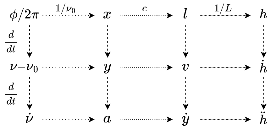
• 信号频率分解：$\displaystyle h(t) = \int \tilde{h}(f) e^{i2\pi f t} df$
• 信号传播时延：$h(t, \vec{r}) = h_{\vec{r}=0}(t-\hat{k}\cdot\frac{\vec{r}}{c})$

取空间任意位置作为参考点(坐标原点)，$\vec{r}$处的引力波信号可表示为：

$$h^{TT}_{ij} (t, \vec{r}) = \bar{h}^{TT}_{ij}\left(t-\hat{k}\cdot{\textstyle\frac{\vec{r}}{c}}\right) = \int\tilde{h}^{TT}_{ij}(f) e^{i 2\pi f (t-\hat{k}\cdot\frac{\vec{r}}{c})} df$$

这里 $\bar{h}_{ij}$ 为原点处($\vec{r}=0$)的引力波信号，而 $\tilde{h}_{ij}(f)$ 为其傅里叶变换。注意，一般地，$\tilde{h}(f) = \left|\tilde{h}(f)\right|e^{i\phi_0}$是复值函数。

$$e^{i 2\pi f (t-\hat{k}\cdot\frac{\vec{r}}{c})} ~~~~~ {\rm v.s.} ~~~~~~ e^{-i 2\pi f (t-\hat{k}\cdot\frac{\vec{r}}{c})}$$

下面考虑激光沿干涉臂传播过程中受到的影响，为便于推导这里先关注单个频率成分：

$$\Delta t = \frac{1}{2c}\int_{s=0}^{L} h(s) d s= \frac{1}{2c}\int_{s=0}^{L} \hat{x}^i\hat{x}^j \tilde{h}_{ij}(f) e^{i\omega (t-\hat{k}\cdot\frac{\vec{r}}{c})} ds$$

其中，$\vec{r}$ 和 $t$对参量$s$ 的依赖关系由激光传播决定：

$$t(s) = t|_{\vec{r}_1} + s/c = t|_{\vec{r}_2} - L/c + s/c; ~~~ \vec{r}(s) = \vec{r}_1 + s\hat{x} = \vec{r}_2 - L\hat{x} + s\hat{x}$$

这里$\vec{r_1}, \vec{r_2}$分别为激光发射端与接收端，$\hat{x}$由激光发射端指向接收端，$t|_{\vec{r}_1}, t|_{\vec{r}_2}$ 分别为激光发射和接收时刻。注意，上式中只出现了$\hat{x}$而没有$\hat{k}$，因为上述关系完全由激光传播决定，而与引力波无关，激光是沿$\hat{x}$传播。

$$\begin{aligned} \Delta t &= \frac{1}{2c}\hat{x}^i\hat{x}^j \tilde{h}_{ij}(f) \int_{s=0}^{L} e^{i\omega (t|_{\vec{r}_1} + \frac{s}{c} - \hat{k}\cdot\frac{\vec{r}_1}{c} - \hat{k}\cdot\hat{x}\frac{s}{c})} ds\\ &= \frac{1}{2c}\hat{x}^i\hat{x}^j \tilde{h}_{ij}(f) e^{i\omega (t|_{\vec{r}_1} - \hat{k}\cdot\frac{\vec{r}_1}{c})} \int_{s=0}^{L} e^{i\omega (1 - \hat{k}\cdot\hat{x})\frac{s}{c}} ds\\ &= \frac{1}{2c}\hat{x}^i\hat{x}^j \tilde{h}_{ij}(f) e^{i\omega (t|_{\vec{r}_1} - \hat{k}\cdot\frac{\vec{r}_1}{c})} {\small \frac{c}{i\omega (1 - \hat{k}\cdot\hat{x})} } e^{i\omega (1 - \hat{k}\cdot\hat{x})\frac{s}{c}}\Big|_0^L\\ &= \frac{1}{2}\hat{x}^i\hat{x}^j \tilde{h}_{ij}(f) e^{i\omega (t|_{\vec{r}_1} - \hat{k}\cdot\frac{\vec{r}_1}{c})} \small \frac{1}{i\omega (1 - \hat{k}\cdot\hat{x})} \left[e^{i\omega (1 - \hat{k}\cdot\hat{x})\frac{L}{c}}-1\right]\\ &= \frac{1}{2}\hat{x}^i\hat{x}^j \tilde{h}_{ij}(f) e^{i\omega (t|_{\vec{r}_1} - \hat{k}\cdot\frac{\vec{r}_1}{c})} e^{i\omega (1 - \hat{k}\cdot\hat{x})\frac{2L}{c}} ~ \small \frac{2\sin\left[\omega(1-\hat{k} \cdot \hat{x}) \frac{L}{2c}\right] }{\omega(1-\hat{k} \cdot \hat{x})}\\ &= \frac{1}{2}\hat{x}^i\hat{x}^j \tilde{h}_{ij}(f) e^{i\omega (t|_{\vec{r}_1} - \hat{k}\cdot\frac{\vec{r}_1}{c})} e^{i\omega (1-\hat{k} \cdot \hat{x}) \frac{L}{2c}} ~{\small \frac{L}{c}} ~ {\rm sinc}\left[\omega(1-\hat{k} \cdot \hat{x}) {\textstyle \frac{L}{2c}}\right]\\ &= \frac{1}{2}\hat{x}^i\hat{x}^j \tilde{h}_{ij}(f) e^{i\omega (t|_{\vec{r}_1} + \frac{L}{2c} - \hat{k}\cdot\frac{\vec{r}_1+ L\hat{x}/2}{c})} ~{\small \frac{L}{c}} ~ {\rm sinc}\left[\omega(1-\hat{k} \cdot \hat{x}) {\textstyle \frac{L}{2c}}\right]\\ \end{aligned}$$

这里的sinc可以通过窗函数积分直接看出来吗$\frac{1}{2\delta}\int_{-\delta}^{\delta} e^{-ix} dx= {\rm sinc} \delta$

这里$t|_{\vec{r}_1} + \frac{L}{2c}$ 对应激光传播到干涉臂中间的时间，$\vec{r}_1+ L\hat{x}/2$ 则为对应的位矢。因此对于单频引力波，单向传播的激光受到的总影响正比于干涉臂中间时的应变强度乘以${\rm sinc}$项，高频信号受到压制。${\rm sinc}$项傅里叶逆变换为$\rm rect$函数，乘积变卷积。

$$\begin{aligned} \Delta t (t|_{\vec{r}_1}) &= \frac{1}{2}\hat{x}^i\hat{x}^j h_{ij}(t|_{\vec{r}_1} + {\textstyle \frac{L}{2c}}, \vec{r}_1+ {\textstyle \frac{L\hat{x}}{2}}) * \frac{L}{c} \frac{ {\rm rect}\left[ \frac{1}{(1-\hat{k}\cdot\hat{x})\frac{L}{c}} t|_{\vec{r}_1} \right] }{(1-\hat{k}\cdot\hat{x})\frac{L}{c}}\\ &= \frac{1}{2} \frac{ \hat{x}^i\hat{x}^j }{1-\hat{k}\cdot\hat{x}} h_{ij}(t|_{\vec{r}_1} + {\textstyle \frac{L}{2c}}, \vec{r}_1+ {\textstyle \frac{L\hat{x}}{2}}) * {\rm rect}\small \left(\frac{ct|_{\vec{r}_1}/L}{1-\hat{k}\cdot\hat{x}}\right) \end{aligned}$$

引力波信号与矩形窗卷积，相当于信号的滑动平均，窗口宽度为$(1-\hat{k}\cdot\hat{x})\frac{L}{c}$，高频信号相互抵消，响应减弱。

代入$t|_{\vec{r}_1} = t|_{\vec{r}_2} - \frac{L}{c}, \vec{r}_1 = \vec{r}_2 - L\hat{x}$，用接收端的时间和位矢表示有：

$$\begin{aligned} \Delta t &= \frac{1}{2}\hat{x}^i\hat{x}^j \tilde{h}_{ij}(f) e^{i\omega (t|_{\vec{r}_2} - \frac{L}{c} - \hat{k}\cdot\frac{\vec{r}_2}{c} + \hat{k}\cdot\hat{x}\frac{L}{c})} \small \frac{1}{i\omega (1 - \hat{k}\cdot\hat{x})} \left[e^{i\omega (1 - \hat{k}\cdot\hat{x})\frac{L}{c}}-1\right]\\ &= \frac{1}{2}\hat{x}^i\hat{x}^j \tilde{h}_{ij}(f) e^{i\omega (t|_{\vec{r}_2} - \hat{k}\cdot\frac{\vec{r}_2}{c})} \small \frac{1}{i\omega (1 - \hat{k}\cdot\hat{x})} \left[1 - e^{-i\omega (1 - \hat{k}\cdot\hat{x})\frac{L}{c}}\right]\\ &= \frac{1}{2}\hat{x}^i\hat{x}^j \tilde{h}_{ij}(f) e^{i\omega (t|_{\vec{r}_2} - \hat{k}\cdot\frac{\vec{r}_2}{c})} e^{-i\omega (1- \hat{k} \cdot \hat{x}) \frac{L}{2c} } ~ {\small \frac{L}{c}} ~ {\rm sinc}\left[\omega(1-\hat{k} \cdot \hat{x}) {\textstyle \frac{L}{2c}}\right]\\ &= \frac{1}{2}\hat{x}^i\hat{x}^j \tilde{h}_{ij}(f) e^{i\omega (t|_{\vec{r}_2} - \frac{L}{2c} - \hat{k}\cdot\frac{\vec{r}_2-L\hat{x}/2}{c})} ~ {\small \frac{L}{c}} ~ {\rm sinc}\left[\omega(1-\hat{k} \cdot \hat{x}) {\textstyle \frac{L}{2c}}\right] \end{aligned}$$

除了时间(相位)变化，对引力波效应的另一个常用描述是分数多普勒频移$\frac{\Delta \nu}{\nu} = \frac{\nu_{\rm recv} - \nu_{\rm emit}}{\nu_{\rm emit}}$。PTA相关文献中通常记为符号$z$，而在空间引力波探测中更常用$y$表示。根据相位关系：

$$\phi_{\rm recv} = \phi_{\rm emit} + 2 \pi \nu_{\rm emit}\frac{L}{c} + 2 \pi \nu_{\rm emit}\Delta t$$

求导可得$\frac{\Delta \nu}{\nu} = \dot{\Delta t} = i\omega \Delta t$，从而：

$$\begin{aligned} \Delta t &= \frac{1}{2}\hat{x}^i\hat{x}^j \tilde{h}_{ij}(f) e^{i\omega (t|_{\vec{r}_1} + \frac{L}{2c} - \hat{k}\cdot\frac{\vec{r}_1+ L\hat{x}/2}{c})} ~{\small \frac{L}{c}} ~ {\rm sinc}\left[\omega(1-\hat{k} \cdot \hat{x}) {\textstyle \frac{L}{2c}}\right]\\ \frac{\Delta \nu}{\nu} &= \frac{i}{2}\hat{x}^i\hat{x}^j \tilde{h}_{ij}(f) e^{i\omega (t|_{\vec{r}_1} + \frac{L}{2c} - \hat{k}\cdot\frac{\vec{r}_1+ L\hat{x}/2}{c})} ~{\small \frac{\omega L}{c}} ~ {\rm sinc}\left[\omega(1-\hat{k} \cdot \hat{x}) {\textstyle \frac{L}{2c}}\right] \end{aligned}$$

$$\begin{aligned} \Delta t &= \frac{1}{2}\hat{x}^i\hat{x}^j \tilde{h}_{ij}(f) e^{i\omega (t|_{\vec{r}_1} - \hat{k}\cdot\frac{\vec{r}_1}{c})} \small \frac{1}{i\omega (1 - \hat{k}\cdot\hat{x})} \left[e^{i\omega (1 - \hat{k}\cdot\hat{x})\frac{L}{c}}-1\right]\\ \frac{\Delta \nu}{\nu} &= \frac{\hat{x}^i\hat{x}^j}{2 (1 - \hat{k}\cdot\hat{x})} \tilde{h}_{ij}(f) e^{i\omega (t|_{\vec{r}_1} - \hat{k}\cdot\frac{\vec{r}_1}{c})} \left[e^{i\omega (1 - \hat{k}\cdot\hat{x})\frac{L}{c}}-1\right]\\ & = \frac{\hat{x}^i\hat{x}^j}{2(1 - \hat{k}\cdot\hat{x})} \left[\tilde{h}_{ij}(f)e^{i\omega (t|_{\vec{r}_1}+\frac{L}{c} - \hat{k}\cdot\frac{\vec{r}_1 + L\hat{x}}{c}) } - \tilde{h}_{ij}(f)e^{i\omega (t|_{\vec{r}_1} - \hat{k}\cdot\frac{\vec{r}_1}{c})} \right]\\ & = \frac{\hat{x}^i\hat{x}^j}{2(1 - \hat{k}\cdot\hat{x})} \left[\tilde{h}_{ij}(f)e^{i\omega (t|_{\vec{r}_2} - \hat{k}\cdot\frac{\vec{r}_2}{c}) } - \tilde{h}_{ij}(f)e^{i\omega (t|_{\vec{r}_1} - \hat{k}\cdot\frac{\vec{r}_1}{c})} \right] \end{aligned}$$

傅里叶逆变换

$$\boxed{\begin{aligned} y(t) &= \frac{\hat{x}^i\hat{x}^j}{2(1 - \hat{k}\cdot\hat{x})} \left[ h_{ij}(t|_{\vec{r}_2}, \vec{r}_2) - h_{ij}(t|_{\vec{r}_1}, \vec{r}_1) \right] \end{aligned}}$$

这里$\vec{r_1}, \vec{r_2}$分别对应激光发射端与接收端，$t|_{\vec{r}_1}, t|_{\vec{r}_2}$ 则对应激光的发射和接受时间。即，引力波导致的多普勒频移仅由接收时刻(接收端)与发射时刻(发射端)的应变强度之差决定！注意这里$\hat{x}$由激光发射端指向接收端，在PTA相关文献中更常见的是：

$$\begin{aligned} z(t) = \frac{\hat{x}^i\hat{x}^j}{2(1 + \hat{k}\cdot\hat{x})} \left[ h_{ij}(t|_{\vec{r}_2}, \vec{r}_2) - h_{ij}(t|_{\vec{r}_1}, \vec{r}_1) \right] \end{aligned}$$

形式上差了个负号，实际上没有区别，只是这里$\hat{x}$由接收端(地球)指向发射端(脉冲星)。

两种时间基准下，频移的定义还是一样的吗？？

$$\frac{\nu_{\rm recv}-\nu(t)|_{\rm em}}{\nu(t)|_{\rm em}}?? ~~~~\frac{\nu_{\rm recv}-\nu(t)|_{\rm em}}{\nu(t)_{\rm recv}}??$$

$$\begin{aligned} z(t) &\equiv \frac{\nu(t)|_{\rm recv}-\nu_{\rm em}}{\nu_{\rm em}} = \frac{1}{2} \frac{\hat{x}^i\hat{x}^j}{1 + \hat{k}\cdot\hat{x}} \Big[h_{ij}(t) - h_{ij}(t - {\textstyle \frac{L}{c}})\Big] \\ &= \frac{1}{2} \sum_P \frac{\hat{x}^i\hat{x}^j}{1 + \hat{k}\cdot\hat{x}} e^P_{ij} \Big[h_P(t) - h_P(t - {\textstyle \frac{L}{c}})\Big] \end{aligned}$$

其中$\hat{x}$为激光传播方向，$\hat{k}$为引力波传播方向，中括号中前后两项分别为激光接收端和发射端的引力波信号，注意这里只是单臂、单向的响应，后面仪器响应部分有具体推导。对于脉冲星计时(或单向多普勒)测量，对应的就是单臂、单向测量，$\hat{x}$对应脉冲星方位，前一项被称为地球项(Earth term)，后一项被称为脉冲星项(Pulsar term)。如果忽略脉冲星项，$\frac{1}{2}\frac{\hat{x}^i\hat{x}^j}{1 + \hat{k}\cdot\hat{x}} e^P_{ij}$就是通常的脉冲星计时测量对不同引力波极化模式的响应函数。

上面公式均以接收端端时间为基准进行测量，另一种形式是以发射端时间为基准，会出现在往返双向测量中，如激光干涉或双向多普勒追踪。注意前面分母中正负号的变化。

$$z(t) \equiv \frac{\nu(t)-\nu_0}{\nu_0} ?? \frac{\nu_{\rm recv}-\nu(t)|_{\rm em}}{\nu(t)|_{\rm em}}?? = \frac{1}{2} \frac{\hat{x}^i\hat{x}^j}{1 - \hat{k}\cdot\hat{x}} \Big[h_{ij}(t+{\textstyle \frac{L}{c}}) - h_{ij}(t)\Big]$$

除了这里通过对光子路径积分获得距离变化，对应相位改变，求导可得到频率变化。还可以直接推导频率影响，之后积分得到相位改变。
高阶速度项的影响可忽略(Cornish & Rubbo 2003)

以激光发射端为参考

$$\begin{aligned} \Delta t &= \frac{1}{2}\hat{x}^i\hat{x}^j \tilde{h}_{ij}(f) e^{i\omega (t|_{\vec{r}_1} - \hat{k}\cdot\frac{\vec{r}_1}{c})} \small \frac{1}{i\omega (1 - \hat{k}\cdot\hat{x})} \left[e^{i\omega (1 - \hat{k}\cdot\hat{x})\frac{L}{c}}-1\right]\\ &= \frac{1}{2}\hat{x}^i\hat{x}^j \tilde{h}_{ij}(f) e^{i\omega (t|_{\vec{r}_1} - \hat{k}\cdot\frac{\vec{r}_1}{c})} e^{i\omega (1-\hat{k} \cdot \hat{x}) \frac{L}{2c}} ~\small \frac{L}{c} ~ {\rm sinc}\left[\omega(1-\hat{k} \cdot \hat{x}) {\textstyle \frac{L}{2c}}\right]\\ \frac{\Delta \nu}{\nu} &= \frac{\hat{x}^i\hat{x}^j}{2 (1 - \hat{k}\cdot\hat{x})} \tilde{h}_{ij}(f) e^{i\omega (t|_{\vec{r}_1} - \hat{k}\cdot\frac{\vec{r}_1}{c})} \left[e^{i\omega (1 - \hat{k}\cdot\hat{x})\frac{L}{c}}-1\right]\\ & = \frac{\hat{x}^i\hat{x}^j}{2(1 - \hat{k}\cdot\hat{x})} \left[\tilde{h}_{ij}(f)e^{i\omega [t|_{\vec{r}_2} - \hat{k}\cdot\frac{\vec{r}_2}{c}] } - \tilde{h}_{ij}(f)e^{i\omega (t|_{\vec{r}_1} - \hat{k}\cdot\frac{\vec{r}_1}{c})} \right] \end{aligned}$$

取发射端为原点，$\vec{r}_1 = 0$

$$\begin{aligned} \Delta t &= \frac{1}{2}\frac{L}{c}\hat{x}^i\hat{x}^j \tilde{h}_{ij}(f) e^{i\omega t} e^{i\omega (1-\hat{k} \cdot \hat{x}) \frac{L}{2c}} ~ {\rm sinc}\left[\omega(1-\hat{k} \cdot \hat{x}) {\textstyle \frac{L}{2c}}\right]\\ \frac{\Delta \nu}{\nu} &= \frac{\hat{x}^i\hat{x}^j}{2 (1 - \hat{k}\cdot\hat{x})} \tilde{h}_{ij}(f) e^{i\omega t} \left[e^{i\omega (1 - \hat{k}\cdot\hat{x})\frac{L}{c}}-1\right] \end{aligned}$$

以激光接收端为参考，$\hat{x}$ 反向(指向发射端)

$$\begin{aligned} \Delta t &= \frac{1}{2}\hat{x}^i\hat{x}^j \tilde{h}_{ij}(f) e^{i\omega (t|_{\vec{r}_2} - \hat{k}\cdot\frac{\vec{r}_2}{c})} \small \frac{1}{i\omega (1 - \hat{k}\cdot\hat{x})} \left[1 - e^{-i\omega (1 - \hat{k}\cdot\hat{x})\frac{L}{c}}\right]\\ &= \frac{1}{2}\hat{x}^i\hat{x}^j \tilde{h}_{ij}(f) e^{i\omega (t|_{\vec{r}_2} - \hat{k}\cdot\frac{\vec{r}_2}{c})} e^{-i\omega (1- \hat{k} \cdot \hat{x}) \frac{L}{2c} } ~ \small \frac{L}{c} ~ {\rm sinc}\left[\omega(1-\hat{k} \cdot \hat{x}) {\textstyle \frac{L}{2c}}\right]\\ \frac{\Delta \nu}{\nu} &= \frac{\hat{x}^i\hat{x}^j}{2 (1 + \hat{k}\cdot\hat{x})} \tilde{h}_{ij}(f) e^{i\omega (t|_{\vec{r}_2} - \hat{k}\cdot\frac{\vec{r}_2}{c})} \left[1 - e^{-i\omega (1 + \hat{k}\cdot\hat{x})\frac{L}{c}}\right]\\ & = \frac{\hat{x}^i\hat{x}^j}{2(1 + \hat{k}\cdot\hat{x})} \left[\tilde{h}_{ij}(f) e^{i\omega (t|_{\vec{r}_2} - \hat{k}\cdot\frac{\vec{r}_2}{c})} - \tilde{h}_{ij}(f) e^{i\omega (t|_{\vec{r}_1} - \hat{k}\cdot\frac{\vec{r}_1}{c}) } \right] \end{aligned}$$

取接收端为原点，$\vec{r}_2 =0$

$$\begin{aligned} \Delta t &= \frac{1}{2}\frac{L}{c}\hat{x}^i\hat{x}^j \tilde{h}_{ij}(f) e^{i\omega t} e^{-i\omega (1+ \hat{k} \cdot \hat{x}) \frac{L}{2c} } ~ {\rm sinc}\left[\omega(1+\hat{k} \cdot \hat{x}) {\textstyle \frac{L}{2c}}\right]\\ \frac{\Delta \nu}{\nu} &= \frac{\hat{x}^i\hat{x}^j}{2 (1 + \hat{k}\cdot\hat{x})} \tilde{h}_{ij}(f) e^{i\omega t} \left[1 - e^{-i\omega (1 + \hat{k}\cdot\hat{x})\frac{L}{c}}\right] \end{aligned}$$

最后，对于单臂往返，发射与接收端重合，将最终接收时间$t_{\rm recv}$简记为$t$，考虑往返的总效应，有：

$$\begin{aligned} \Delta t &= \frac{1}{2}\hat{x}^i\hat{x}^j \tilde{h}_{ij}(f) e^{i\omega (t - \hat{k}\cdot\frac{\vec{r}_1}{c})} \small \frac{1}{i\omega (1 + \hat{k}\cdot\hat{x})} \left[1 - e^{-i\omega (1 + \hat{k}\cdot\hat{x})\frac{L}{c}}\right]\\ &~~~~~ + \frac{1}{2}\hat{x}^i\hat{x}^j \tilde{h}_{ij}(f) e^{i\omega (t - \frac{2L}{c} - \hat{k}\cdot\frac{\vec{r}_1}{c})} \small \frac{1}{i\omega (1 - \hat{k}\cdot\hat{x})} \left[e^{i\omega (1 - \hat{k}\cdot\hat{x})\frac{L}{c}}-1\right]\\ &= \frac{1}{2}\hat{x}^i\hat{x}^j \tilde{h}_{ij}(f) e^{i\omega (t - \hat{k}\cdot\frac{\vec{r}_1}{c})} \small \frac{1}{i\omega} \left[ \frac{1 - e^{-i\omega (1 + \hat{k}\cdot\hat{x})\frac{L}{c}}}{1 + \hat{k}\cdot\hat{x}} + e^{-i\omega \frac{2L}{c}} \frac{e^{i\omega (1 - \hat{k}\cdot\hat{x})\frac{L}{c}}-1}{1 - \hat{k}\cdot\hat{x}}\right]\\ &= \frac{1}{2}\hat{x}^i\hat{x}^j \tilde{h}_{ij}(f) e^{i\omega (t - \hat{k}\cdot\frac{\vec{r}_1}{c})} {\small \frac{L}{c}} \bigg\{ e^{-i\omega (1 + \hat{k}\cdot\hat{x})\frac{L}{2c}} ~ {\rm sinc}\left[\omega (1 + \hat{k}\cdot\hat{x}) {\textstyle \frac{L}{2c}}\right] \\ & ~~~~~~~~~~~~~~~~~~~~~~~~~~~~~~~~~~~~~~~~~~~~~~ + e^{-i\omega (3+\hat{k} \cdot \hat{x}) \frac{L}{2c}} ~ {\rm sinc}\left[\omega (1 - \hat{k}\cdot\hat{x}) {\textstyle \frac{L}{2c}}\right]\bigg\} \end{aligned}$$

将大括号内部分记为$\mathcal{T}(f, \hat{k} \cdot \hat{x})$，同时引入特征频率$f_*=\frac{c}{2L}$，有：

$$\boxed{\begin{aligned} \Delta t &= \frac{1}{2}\hat{x}^i\hat{x}^j \tilde{h}_{ij}(f) e^{i\omega (t - \hat{k}\cdot\frac{\vec{r}_1}{c})} \frac{L}{c} \mathcal{T}(f, \hat{k} \cdot \hat{x})\\ \small\mathcal{T}(f, \hat{k} \cdot \hat{x}) &\equiv \small e^{-i\pi (3+\hat{k} \cdot \hat{x}) \frac{f}{2f_*}} ~ {\rm sinc}\left[\pi(1-\hat{k} \cdot \hat{x}) {\textstyle \frac{f}{2f_*}}\right] + e^{-i\pi(1+\hat{k} \cdot \hat{x}) \frac{f}{2f_*}} ~ {\rm sinc}\left[\pi(1+\hat{k} \cdot \hat{x}) {\textstyle \frac{f}{2f_*}}\right]\\ &= \small \left\{e^{-i\pi \frac{f}{2f_*}} ~ {\rm sinc}\left[\pi(1-\hat{k} \cdot \hat{x}) {\textstyle \frac{f}{2f_*}}\right] + e^{i\pi \frac{f}{2f_*}} ~ {\rm sinc}\left[\pi(1+\hat{k} \cdot \hat{x}) {\textstyle \frac{f}{2f_*}}\right]\right\} e^{-i\pi(2 + \hat{k} \cdot \hat{x})\frac{f}{2f_*}} \end{aligned}}$$

一些文章将$\mathcal{T}(f, \hat{k} \cdot \hat{x})$称为转移函数(transfer function)，但这并不准确，转移函数通常指系统的响应函数(response function)，应包含天线指向性函数，Schilling 1997中的形式就是包含的，后面具体分析。
对于一般的n次往返情况，上式中$e^{-i\pi(2 + \hat{k} \cdot \hat{x})\frac{f}{2f_*}}$变为$e^{-i\pi 2n\frac{f}{2f_*}} \frac{\sin(2n\pi\frac{f}{2f_*})}{n\sin(2\pi\frac{f}{2f_*})}$，而对于地面引力波探测的Fabry-Perot腔，响应是多次往返之和，大致接近多次往返响应函数的包络线，具体可参考Schilling 1997。

如果将上述时间变化量转换为对应的无量纲应变响应，有：

$$\begin{aligned} s(f, t, \hat{x}, \hat{k}, \vec{r}_1) &\equiv {\small \frac{\Delta L}{L}} = {\small \frac{c \Delta t}{L}} = \frac{1}{2}\hat{x}^i\hat{x}^j \tilde{h}_{ij}(f)e^{i 2\pi f (t - \hat{k}\cdot\frac{\vec{r}_1}{c})} ~\mathcal{T}(f, \hat{k} \cdot \hat{x}) \end{aligned}$$

$s(f,t)$就是激光臂对单个频率成分 $\tilde{h}_{ij}(f)e^{i\omega t}$ 的响应，其中 $e^{-i 2\pi f \hat{k}\cdot\frac{\vec{r}_1}{c})}$ 项为引力波由参考系原点至测量点的传播延迟，下一小节具体讨论，这里暂时忽略。可以看到响应是线性的，即$s \propto \tilde{h}_{ij}(f)e^{i\omega t}$，因此总的引力波响应就是所有频率分量贡献的线性叠加，即对频率积分。用$\mathscr{D}$表示探测器响应：

$$\begin{aligned} s(t) &= \mathscr{D}\left(h_{ij}(t)\right) = \mathscr{D}\left(\int \tilde{h}_{ij}(f)e^{i 2\pi f t} df\right)\\ &= \int \mathscr{D}\left(\tilde{h}_{ij}(f)e^{i 2\pi f t}\right) df = \int s(f, t) df\\ &= \int df ~ \frac{1}{2}\hat{x}^i\hat{x}^j \tilde{h}_{ij}(f)e^{i 2\pi f t} ~\mathcal{T}(f, \hat{k} \cdot \hat{x})\\ &= \int \left[ \frac{1}{2}\hat{x}^i\hat{x}^j \tilde{h}_{ij}(f)~\mathcal{T}(f, \hat{k} \cdot \hat{x})\right] ~e^{i 2\pi f t} df \end{aligned}$$

$$\begin{aligned} \tilde{s}(f) &= \mathcal{F}\left\{s(t)\right\} = \frac{1}{2}\hat{x}^i\hat{x}^j \tilde{h}_{ij}(f) \mathcal{T}(f, \hat{k} \cdot \hat{x}) \end{aligned}$$

定义系统的转移函数

$$F^P(f) = \frac{1}{2}\hat{x}^i \hat{x}^j e_{ij}^P~\mathcal{T}(f, \hat{k} \cdot \hat{x})$$

从而对频域信号：

$$\tilde{s}(f) = F^P(f) \tilde{h}_P(f) = F^+(f)\tilde{h}_+(f) + F^\times(f)\tilde{h}_\times(f)$$

至此，考虑的还只是单臂往返的响应，对于双臂干涉情况，系统转移函数为：

$$\boxed{F^P(f) = \frac{1}{2}\left[\hat{x}^i \hat{x}^j e_{ij}^P~\mathcal{T}(f, \hat{k} \cdot \hat{x}) - \hat{y}^i \hat{y}^j e_{ij}^P~\mathcal{T}(f, \hat{k} \cdot \hat{y})\right]}$$

$$\boxed{D^P(f) = D^{ij} e_{ij}^P; ~~~ D^{ij} = \frac{1}{2}\left[\hat{x}^i \hat{x}^j ~\mathcal{T}(f, \hat{k} \cdot \hat{x}) - \hat{y}^i \hat{y}^j ~\mathcal{T}(f, \hat{k} \cdot \hat{y})\right]}$$

在长波近似下，$\mathcal{T}(f, \theta, \varphi) \sim 1$，转移函数$F^P(t)$不含时，卷积退化为普通乘积，而此时$F^P$则对应前面的天线模式函数。
同时对于单频信号$\tilde{h}_P(f)$ 为 $\delta$ 函数，
注意这里没有考虑探测器轨道运动，时域$\delta$ 函数？

常见的，依然是频域函数，是

$$s(t) = F^P h_P(t) = F^+ h_+(t) + F^\times h_\times(t)$$

长波极限近似
把所有包含引力波传播($\hat{k}$)的项忽略即可得到长波近似结果，剩余的时间差异，仅由激光传播引入！

地面探测器处于长波极限(L ≪ λ)，可以将整个探测器作为参考系。
但对于空间探测器，长波极限近似不再始终成立，计算探测器响应时必须考虑，信号在探测器中的传播时间，以及探测器响应的时间延迟。

不但不满足长波近似，考虑到超长的臂长必须考虑光传播的时间，其中之一就是在发射激光时不是指向卫星当前位置，而是约8s(L/c)之后的位置，需在不引入额外光程及抖动限制下，对反射镜指向进行超前瞄准调控。

探测器运动调制

对于地基探测器，存在地球自转和公转
对于空间探测器，同样存在探测器的自转和公转

通常波源位置会通过赤道或黄道天球坐标描述，而空间探测中探测器位于地球公转轨道，信号投影时需要通过黄道天球坐标系建立波源与探测的联系。考虑到探测器的公转及自转，信号的投影也将随时间演化。此外，探测器的轨道运动本身(非惯性系)，还将在信号中引入额外调制。

坐标变换
波源参考系
探测器参考系
赤道参考系/黄道参考系
从波源到黄道、从黄道到探测器？？？

信号调制(多普勒调制)
从太阳系质心SSB到探测器，而且随着探测器运动，信号延迟(或提前)时间周期性变化
多普勒调制

$$\bm{h}_{\rm det}(t) = \bm{h}_{\rm \tiny SSB}\left(t - \hat{k}\cdot\frac{\vec{r}_{\rm det}}{c}\right) = \bm{h}_{\rm \tiny SSB}(t) e^{- i\omega\hat{k}\cdot\frac{\vec{r}_{\rm det}}{c}}$$

噪声与灵敏度

前面的信噪比分析主要涉及信号的(功率)响应以及噪声功率谱，信号响应前面章节已经讨论过，本节的关注点是探测器的噪声分析。

噪声转换

空间测量中存在多种噪声，表现形式涉及位移$l$、相位$\phi$、频率$\nu$、速度$v$、加速度$a$等各种物理量，这里基于物理量间的时域关系，分析频域中不同量纲噪声功率谱间的转换关系。
以下将用$\nu$表示信号载波(如激光)频率，考虑到频率波动，载波的中心基准频率和波长记为$\nu_0, \lambda_0$。作为区分，噪声数据傅里叶变换的频域，对应于引力波频率，用$f$表示，$\omega, \lambda_{\rm GW}$分别表示引力波角频率和波长。

涉及到的物理量之间的转换

用于测量的激光信号可用电场强度表征：

$$E(t) = E_0(t) e^{j\varphi(t)} = E_0(t) e^{j[2\pi\nu_0 t + \phi(t)]}$$

这里$E_0(t)$为信号的(瞬时)振幅，受激光功率不稳定影响，振幅存在波动；$\varphi(t)$为信号的瞬时相位，其导数为瞬时角频率。$\nu_0$为激光的中心频率，$\phi(t)$则是瞬时相位$\varphi(t)$相对线性增长的基准相位$2\pi\nu_0 t$的波动残差。主要的噪声以及引力波信号都位于$\phi(t)$中。

$$\omega(t) = \dot{\varphi}(t), ~~~ \nu(t) = \frac{\dot{\varphi}(t)}{2\pi} = \nu_0 + \frac{\dot{\phi}(t)}{2\pi}; ~~~ \varphi(t) = 2\pi \int_{t_0}^t\nu(\tau)d\tau$$

除了相位与频率外，另两个常用的描述相位演化的物理量是计时抖动(timing jitter)$x(t)$及其导数——相对频偏(relative frequency deviation)或分数多普勒频移(fractional doppler shift)$y(t)$。其中计时抖动是以中心频率$\nu_0$作为基准，将相位残差$\phi(t)$转换为时间，反映了瞬时相位$\varphi(t)$所对应的时间与实际(线性)时间之间的偏离，即所谓抖动，其导数对应于激光瞬时频率$\nu(t)$与中心频率$\nu_0$的相对偏离。

$$x(t) = \frac{\phi(t)}{2\pi\nu_0} = \frac{\varphi(t)}{2\pi\nu_0} - t; ~~~~~ y(t) = \dot{x}(t) = \frac{\nu(t)-\nu_0}{\nu_0}$$

• 位移：

  $$h = \frac{l}{L}; ~~~~~~ \sqrt{S_h} = \frac{1}{L}\sqrt{S_l}$$

• 相位：

  $$\phi = 2\pi \nu_0 \frac{l}{c} = 2\pi \frac{l}{\lambda_0}; ~~~ \sqrt{S_l} = \frac{\lambda_0}{2\pi}\sqrt{S_\phi}; ~~~ \sqrt{S_h} = \frac{1}{L} \frac{\lambda_0}{2\pi}\sqrt{S_\phi}$$

• 计时抖动(timing jitter)：

  $$x(t) \equiv \frac{\phi}{2\pi\nu_0} = \frac{l}{c}; ~~~~~ \sqrt{S_l} = c \sqrt{S_x}; ~~~~~ \sqrt{S_h} = \frac{1}{L/c} \sqrt{S_x}$$

• 速度：

  $$v = \dot{l}; ~~~~~~ \sqrt{S_l} = \frac{1}{2\pi f} \sqrt{S_v}; ~~~~~ \sqrt{S_h} = \frac{1}{L} \frac{1}{2\pi f} \sqrt{S_v}$$

• 频率：

  $$\nu = \nu_0 + \frac{\dot{\phi}}{2\pi}; ~~~~~ \sqrt{S_\phi} = \frac{1}{f} \sqrt{S_\nu}; ~~~~~ \sqrt{S_h} = \frac{1}{L} \frac{\lambda_0}{2\pi f} \sqrt{S_\nu}$$

  $$\nu = \nu_0 + \frac{\dot{\phi}}{2\pi} = (1+\frac{v}{c})\nu_0; ~~~ v = c\frac{\nu-\nu_0}{\nu_0}; ~~~ \sqrt{S_v} = \lambda_0 \sqrt{S_\nu}$$

• 分数频移：

  $$y(t) \equiv \frac{\nu-\nu_0}{\nu_0} = \frac{v}{c}; ~~~ \sqrt{S_\nu} = \nu_0 \sqrt{S_y}; ~~~ \sqrt{S_h} = \frac{1}{L/c} \frac{1}{2\pi f} \sqrt{S_y}$$

• 加速度：

  $$a = \dot{v}; ~~~~~ \sqrt{S_v} = \frac{1}{2\pi f} \sqrt{S_a}; ~~~~~ \sqrt{S_h} = \frac{1}{L} \frac{1}{(2\pi f)^2} \sqrt{S_a}$$

  $$a = \dot{v} = c ~\dot{y} = \frac{c}{\nu_0}\dot{\nu} = \lambda_0\dot{\nu}; ~~~~~~~~ \dot{y} = \frac{\dot{\nu}}{\nu_0} = \frac{a}{c}~~~~~~$$

• 啁啾度(chirpyness)：频率导数
  如上所示，啁啾度与加速度直接对应$\displaystyle \gamma = \dot{\nu} = \frac{1}{\lambda_0}a$，其功率谱较少用到。

注意，这里讨论的都是单程噪声，单臂往返噪声$L$需变为$2L$，同时对于空间观测往返过程的噪声相互独立，对应的应变噪声功率谱$S_h$需乘以2，因此最终$S_h$为上述表达式的$1/2$。

上面各种形式噪声中，位移与相位及计时抖动、速度与频率及分数频移、加速度与频率导数(啁啾度)分别对应，各自间呈简单比例关系，功率谱有相同的频率依赖。三类噪声之间通过求导(积分)转换，对应到频域会出现$2\pi f$项，改变频谱的频率依赖。可以看到与应变幅值谱的转换中，频率、速度和分数频移噪声均出现了$\frac{1}{2\pi f}$，加速度噪声中则出现了$\frac{1}{(2\pi f)^2}$。

$$l = c ~ x = c\frac{\phi}{2\pi\nu_0}; ~~~~~ v= c ~ \dot{x} = c ~ y = c\frac{\nu-\nu_0}{\nu_0}; ~~~~~ a = c ~ \dot{y} = c \frac{\dot{\nu}}{\nu_0}$$

注意，相位、频率及频率导数形式的噪声都依赖于载波(如激光)频率，通过降低基准频率就可降低噪声的绝对数值，相对的，计时抖动和分数频率则约化了基准频率的影响。在讨论相位或频率噪声时，必须给定载波频率才有意义。同时在不同噪声间进行对比或转换时，需根据具体情况选择合适形式。比如对于LISA$~\small L\sim 2.5\times 10^9 {\rm m}, f \sim 1 {\rm mHz}$，应变噪声需求$\small \sqrt{S_h} \sim 10^{-20}/\rm \sqrt{Hz}$，转换为相位噪声$\small \sqrt{S_\phi} \sim 15 \rm \mu rad/\sqrt{Hz} \sim \mu cycle/\sqrt{Hz}$。最终相位测量中，会通过ADC模块对约$\small 20 \rm MHz$的拍频信号进行采样，采样间隔的计时误差显然需要低于LISA需求，注意此时载波信号频率是$\small 20 \rm MHz$，最终对应计时抖动要求为$\small \sqrt{S_x} \sim 10^{-13} \rm s/\sqrt{Hz}$，相对频移$\small \sqrt{S_y} \sim 10^{-15} \rm /\sqrt{Hz}$，相比原始值降了7个量级(载频降低而相位噪声要求不变)。但即便如此，目前的星载时钟仍无法满足需求，实际中会通过时钟间的外差测量进一步降低噪声要求。

此外值得注意的是分数频率，与应变一样，分数频率也是无量纲量，而且两者在量级上也很接近，对空间观测$\small \sqrt{S_h} \sim 20 \sqrt{S_y}$(mHz频段)，地面观测$\small \sqrt{S_h} \sim 1/2 \sqrt{S_y}$(100Hz频段)。空间探测激光频率噪声$\small \sqrt{S_\nu} \sim 30\rm Hz/\sqrt{Hz}$(mHz频段)，基准频率$\small 2.8 \times 10^{14} \rm Hz$(1064nm)，对应通常说的分数频率噪声$\small \sqrt{S_y} \sim 10^{-13}/\sqrt{\rm Hz}$，最终实际应变噪声仅高一个量级$\small \sqrt{S_h} \sim 10^{-12}/\sqrt{\rm Hz}$，很容易被混淆。两者实际物理意义不同，对频率的依赖也不同，注意区分。最后，转换后的应变噪声仍然并非激光不稳定性实际贡献的噪声水平，因为不同臂的激光进行干涉时相位(频率)是相关的。

实际的引力波观测是对两个臂的激光进行干涉，相位作差，上面介绍的转换关系隐含了假设噪声源在干涉测量中独立。尤其是对频率而言，激光内禀的频率噪声不能简单套用上述公式，因为激光频率不稳定性在干涉测量中是相关的。简单的，以臂长不相等的分光干涉为例，干涉测量的相位差：

$$\Delta \phi(t) = \phi(t- \frac{2L_1}{c}) - \phi(t- \frac{2L_2}{c}) = \phi(t- \frac{2L_1}{c}) - \phi(t- \frac{2L_1}{c} + \frac{2\Delta L}{c})$$

其中$\Delta L= L_1 - L_2$为臂长差，对上式进行傅里叶变换，时移对应相移：

$$\widetilde{\Delta \phi}(f) = \tilde{\phi}(f - 2L_1/c) \left(1 - e^{i \omega \frac{2\Delta L}{c}}\right) \approx \tilde{\phi}(f - 2L_1/c) \cdot - i \omega \frac{2\Delta L}{c}$$

取$\small f \sim 1 {\rm mHz}, \Delta L \sim 0.01L = 3\times 10^4 \rm km \sim 0.1 s$，$\small \omega \frac{2\Delta L}{c} = 4\pi f \frac{\Delta L}{c} \sim 10^{-3}$，因此可进行上述近似。同时$\frac{\Delta L}{c} f = \frac{\Delta L}{\lambda_{\rm GW}} \ll 1$也将极大抑制激光本身频率(相位)不稳定性对干涉测量相位差的影响。根据上述傅里叶变换，对应的功率谱：

$$\sqrt{S_{\Delta \phi}} = 4\pi \frac{\Delta L}{c} f \sqrt{S_\phi}, ~~~~~ \sqrt{S_{\Delta \phi}} / \sqrt{S_\phi} = 4\pi \frac{\Delta L}{c} f \sim 10^{-3}\frac{f}{1\rm mHz}$$

由于激光频率噪声的相关性，干涉测量中的残余噪声仅为原始值的千分之一。之后可正常使用前面的噪声转换关系，最终引入的应变噪声与原始噪声谱关系为：

$$\sqrt{S^h_{\rm freq}} = \frac{1}{L} \frac{\lambda_0}{2\pi} \sqrt{S_{\Delta \phi}} = 2 \frac{\Delta L}{L}\frac{f}{\nu_0} \sqrt{S_\phi} = 2 \frac{\Delta L}{L}\frac{1}{\nu_0} \sqrt{S_\nu} = 2 \frac{\Delta L}{L} \sqrt{S_y}$$

实际的空间测量，虽然并非简单的分光干涉，但通过利用外差测量及锁相技术，不同方向上的激光相位同样保持相关，效果上与这里讨论的分光干涉一致。

对$\Delta\phi=2\pi\nu\frac{2\Delta L}{c}$求微分，考虑到频率和臂长都存在波动：

$$\delta\phi = \frac{4\pi}{c}\left(\delta\nu \Delta L + \nu \delta L\right) = \Delta\phi \left(\frac{\delta\nu}{\nu} + \frac{\delta L}{\Delta L}\right)$$

除了上述严格推导，考虑到最终观测量是干涉测量的相位差，粗略地有：

$$\Delta\phi(t) = 2\pi \nu_0\frac{2 \Delta L}{c}$$

注意这里其实已经暗含利用了相位的相关性。对于观测到的相位差而言，频率的相对波动与臂长差的相对波动是无法区分的：

$$\frac{4\pi \nu_0}{c}(1+\frac{\delta \nu}{\nu_0}) \Delta L ~~~ \leftrightarrow ~~~ \frac{4\pi \nu_0}{c}(1+\frac{\delta L}{\Delta L}) \Delta L$$

频率不稳定性可转为为臂长的相对不稳定性，影响最终的引力波应变测量：

$$h \sim \frac{\delta L}{L} \leftrightarrow \frac{\Delta L}{L} \frac{\delta \nu}{\nu_0}$$

从而，激光频率不稳定性所贡献的应变噪声水平为：

$$\sqrt{S_{\rm freq}^h} = \frac{\Delta L}{L} ~ \sqrt{S_y}$$

与前面的分析差了一个2倍，不清楚问题在哪。

最后，简单进行估算，空间探测中激光分数频率噪声$\small \sqrt{S_y} \sim 10^{-13}/\sqrt{\rm Hz}$，实际贡献的噪声水平为$\small \sqrt{S_{\rm freq}^h} \sim 10^{-15}/\sqrt{\rm Hz}$。作为对比，地基探测器通常有几厘米或十厘米的静态臂长差(Schnupp asymmetry)，具体的 aLIGO 为8cm，AdVirgo 为23cm，$\small \frac{\Delta L}{L} \sim 5 \times 10^{-5}$。同时，激光频率不稳定性$\small \sqrt{S_\nu} \sim 10^{-6}{\rm Hz/\sqrt{Hz}}, \sqrt{S_y} \sim 4 \times 10^{-21}\rm Hz/\sqrt{Hz}$(100Hz频段)，最终贡献的噪声水平为$\small \sqrt{S_{\rm freq}^h} \sim 10^{-25}/\rm \sqrt{Hz}$。

地基观测的激光稳定性是满足需求的($\small \sim 10^{-21}$)，但对于空间观测，即便已经降了3个量级，残余频率噪声的影响仍远高于观测需求($\small \sim 10^{-20}$)。地基探测中等效臂长$\small L\sim 1000 \rm km$，臂长差$\small \Delta L\sim 50 \rm m$，干涉测量中噪声被压低约$\small 4\pi \frac{\Delta L}{c} f \sim 2 \times 10^{-4}\frac{f}{100\rm Hz}$，相比空间好一个量级。更主要的差别在于激光本身的不稳定性，空间相比地面差了近8个量级($\small \sim 4\times 10^{-8}$)，这主要是受限于卫星载荷(预算)。FP腔受空间环境的温度波动影响。

为达到与地面相当的噪声水平，相对臂长差需要比地面低7~8个量级，达到$10^{-12}$，相比实际的百分之一量级要降10个量级，这点主要通过时间延迟干涉TDI技术实现。具体的，通过构建虚拟等臂干涉，一代TDI可将臂长残差降低约6个量级$\small \Delta L \sim 10^{-8} L \sim 30\rm m \sim 10^{-7}s$，对应$\small \sqrt{S_{\rm freq}^h} \sim 10^{-21}/\sqrt{\rm Hz}$，已基本满足观测需求。进一步的，通过将空间探测中臂长随卫星运动的动态变化纳入考量，第二代TDI相比一代理论上臂长差可进一步降4个量级，最终$\small \Delta L \sim 10^{-12} L \sim 3\rm mm \sim 10^{-11}s$，$\small \sqrt{S_{\rm freq}^h} \sim 10^{-25}/\sqrt{\rm Hz}$，与地基观测相当。实际中只能做到约3个量级$\small \Delta L \sim 30\rm mm$，$\small \sqrt{S_{\rm freq}^h} \sim 10^{-24}/\sqrt{\rm Hz}$。

噪声曲线

在经过TDI等噪声抑制处理，决定探测器灵敏度的次级噪声主要可分为两种，加速噪声与位移噪声。
加速噪声主要来自测试质量模块，是测试质量受到的静电力、磁力、扭力、分子碰撞、温度梯度及重力变化等各种未能完全屏蔽的外力残余所引入的加速度。加速噪声直接对应频率导数的改变，并最终影响相位测量，转换为位移形式时功率谱需除以$(2\pi f)^4$。
位移噪声则主要来自相位测量端，也被称为读出噪声或光学测量噪声(？)，通常以位移(而非相位)形式描述。其中最核心的是散粒噪声，即由激光功率不稳定性(？)所引入的噪声。散粒噪声属于量子极限噪声，是无法避免的，限制了位移噪声抑制的下限，也限制了整个引力波探测的灵敏度下限。同时值得注意的，散粒噪声为高斯白噪声，取值是不依赖频率的固定值，对应的应变噪声也同样是白噪声。

• 加速噪声(Acceleration Noise)

$$N_{\rm acc}(f)=\left(3 ~ {\rm fm}/s^2/\sqrt{\rm Hz}\right)^2\cdot \small \left[1+\left(\frac{0.4 \rm mHz}{f}\right)^2\right]\cdot\left[1+\left(\frac{f}{8 \rm mHz}\right)^4\right]$$

$$\small \sqrt{N^h_{\rm acc}(f)} = \frac{1}{L} \frac{1}{(2\pi f)^2}\sqrt{S_{\rm acc}(f)} = 4.7\times 10^{-22}/\sqrt{\rm Hz} \sqrt{\footnotesize \left[1+\left(\frac{0.4 \rm mHz}{f}\right)^2\right]\cdot\left[1+\left(\frac{8 \rm mHz}{f}\right)^4\right]}$$

可以看到加速噪声本身，由两项分别在不同频段占据主导：$0.4 \rm mHz$以下$\sqrt{N_{\rm acc}} \propto f^{-1}$，随频率增加而降低，$8 \rm mHz$以上$\propto f^{2}$，随频率增加增大。而对应的应变噪声水平的变化则完全由后一项主导，$8 \rm mHz$以下$\sqrt{N^h_{\rm acc}} \propto f^{-2}$，$8 \rm mHz$以上保持不变。

跟最终灵敏度曲线还差了20/3的常数倍，源自仪器的响应，有待确认

• 位移噪声(Displacement Noise)
  位移噪声或者光学测量系统(Optical Metrology System, OMS)噪声的核心是散粒噪声，以相位形式表示，对应的噪声功率谱密度为：

  $$N^\phi_{\rm shot} = \frac{h\nu_0}{\eta P_{\rm in}}, ~~~ P_{\rm in} = \left(\frac{D^2}{2 \lambda_0 L}\right)^2 P_{\rm E}$$

  $$\sqrt{N^l_{\rm shot}} = \frac{\lambda_0}{2\pi} \sqrt{N^\phi_{\rm shot}} = \frac{\lambda_0^2 L}{\pi D^2} \sqrt{ \frac{h \nu_0}{\eta P_{\rm E}} }$$

  $$\sqrt{N^h_{\rm shot}} = \frac{1}{L} \sqrt{N^l_{\rm shot}} = \frac{\lambda_0^2}{\pi D^2}\sqrt{ \frac{h\nu_0}{\eta P_{\rm E}} }$$

  可见散粒噪声贡献的应变噪声水平仅依赖激光发射功率及望远镜直径，与臂长无关。以LISA为例，激光功率2W、臂长250公里，散粒噪声在$\small 10\rm pm/\sqrt{Hz}$量级，对应的应变噪声约$\small 10^{-21}/\sqrt{\rm Hz}$。作为对比，地面观测散粒噪声可低至$\small 10^{-19} \rm m/\sqrt{Hz}$，空间观测受限于激光(接收)功率，相比地面高了近8个量级。

  $$N^\phi_{\rm shot} = \frac{h\nu_0}{\eta P_{\rm in}}, ~~~ P_{\rm in} = \left(\frac{D^2}{2 \lambda_0 L}\right)^2 P_{\rm E}$$

  $$\sqrt{N^l_{\rm shot}} = \frac{\lambda_0}{2\pi} \sqrt{N^\phi_{\rm shot}} = \frac{\lambda_0^2 L}{\pi D^2} \sqrt{ \frac{h \nu_0}{\eta P_{\rm E}} }$$

  $$\sqrt{N^h_{\rm shot}} = \frac{1}{L} \sqrt{N^l_{\rm shot}} = \frac{\lambda_0^2}{\pi D^2}\sqrt{ \frac{h\nu_0}{\eta P_{\rm E}} }$$

  最后，虽然散粒噪声是白噪声，但考虑到卫星运动等其他因素（？），总的光学测量噪声在低频端并不能达到该极限，仅在高频部分接近白噪声，整体上：

  $$N^l_{\rm OMS} = \left(15 ~ {\rm pm}/\sqrt{\rm Hz}\right)^2 \cdot \left[1+\left(\frac{2 \rm mHz}{f}\right)^4\right]$$

  $$\small \sqrt{N^h_{\rm OMS}} = \frac{1}{L} \sqrt{N^l_{\rm OMS}} = 6\times 10^{-21}/\sqrt{\rm Hz} \cdot \sqrt{1+\left(\frac{2 \rm mHz}{f}\right)^4}$$

L = 2.5e9
D = 0.3
P = 2
c = 3e8
h = 6.626e-34
eta = 0.07
lambda_0 = 1.064e-6
nu_0 = c/lambda_0

1e-6/L/2/np.pi/1e-3*lambda_0

def S_a(f):
  """Returns the value of the function S_a(f)."""
  return (2.4 * 1e-15)**2 * (1 + (0.4 / f)**2) * (1 + (f / 8)**4)

f = np.logspace(-2, 3, 1000) #mHz
S_a_values = S_a(f)


S_h1_root = np.sqrt(S_a_values)/L/(2*np.pi*f*1e-3)**2
# S_h2_root = lambda_0**2/np.pi/D**2 * np.sqrt(h * nu_0/eta/P) # L * S_h2_root
S_h2_root = 1.5e-11/L * np.sqrt(1 + (2/f)**4)

S_h_root = np.sqrt(S_h1_root**2 + S_h2_root**2)


# plt.plot(f, np.sqrt(S_a_values))
plt.plot(f, S_h1_root, '--', color='grey')
plt.plot(f, S_h2_root, '--', color='grey')
plt.plot(f, S_h_root)
plt.xlabel('Frequency (mHz)', fontsize=12)
plt.ylabel('S_a (m/s^2/sqrt(Hz))', fontsize=12)

# Change both axes to log scale
plt.xscale('log')
plt.yscale('log')

plt.show()

灵敏度曲线

$$d(t) = s(t) + n(t), ~s(t) = D^{ab}(t)*h_{ab}(t) = \small \sum_P F^P(t)*h_P(t)$$

变换到频域：

$$\tilde{d}(f) = \tilde{s}(f) + \tilde{n}(f) = \small \sum_P F^P(f) \tilde{h}_P(f) + \tilde{n}(f)$$

对于各向同性无偏振的平稳背景，自相关有

$$\langle\tilde{d}(f)\tilde{d}^*(f)\rangle/T_{\rm obs} = S_h(f) \sum_P |F_P(f)|^2+ N(f) = S_h(f)\mathcal{R}(f) + N(f)$$

在噪声谱已知时，信噪比可表示为：

$$\rho = 2 \int_0^\infty df \frac{S_h(f)\mathcal{R}(f)}{N(f)} = \int_0^\infty df \frac{2 S_h(f)}{N(f)/\mathcal{R}(f)}$$

这里信噪比公式是错的，量纲不对！！Cornish (2002)以及Maggiore书中似乎是逐个频点的，完全不做积分？！

另一方面，对于并和信号匹配滤波，信噪比公式为：

$$\langle\rho^2\rangle = 4 \int_0^\infty df \frac{\langle|\tilde{s}(f)|^2\rangle}{N(f)} = \int_0^\infty df \frac{4\langle|\tilde{h}(f)|^2\rangle}{N(f)/\mathcal{R}(f)}$$

由以上信噪比公式可看出，$N(f)/\mathcal{R}(f)$可作为探测器灵敏度的某种度量。

上面$S_h(f)$或$|\tilde{h}(f)|^2$都对应单个极化模式，当两种偏振模式之和与$N(f)/\mathcal{R}(f)$同一量级时，信噪比分别为1和2。

Babak et al. (2021)定义的灵敏度是$\small N(f)/|F^P(f)|^2$，而此处定义为$\small N(f)/\sum_P |F^P(f)|^2$，两者差了个两倍？？
Robson et al. 2019中$\mathcal{R} = \langle F_+^2\rangle = \langle F_\times^2\rangle$，也是不求和形式！！
Cornish & Larson 2001中是求和的形式！！！

$$\langle\tilde{s}(f)\tilde{s}^*(f)\rangle/T_{\rm obs} = \langle F_+^2\rangle \langle|\tilde{h}_\times|^2 + |\tilde{h}_\times|^2\rangle = \langle|\tilde{h}|^2\rangle \langle F_+^2 + F_\times^2\rangle$$

• 臂长制约(Length Penalty)：受限于臂长，探测器在高频端的响应逐渐衰降

$$\mathcal{R}(f) \approx \frac{3}{10} \frac{1}{1+0.6(\pi f/f_*)^2} \approx \frac{3}{10} \frac{1}{1+ 6(f/f_*)^2}, ~~ f_* = \frac{c}{2L}$$

$$\mathcal{R}(f) = \frac{3}{10} \frac{1}{1+(f/25\rm mHz)^2}$$

这里不同于Robson et al. 2019，特征频率取为$\frac{c}{2L}$而非$\frac{c}{2\pi L}$，相应的分母中0.6变为$0.6\pi^2 \sim 6$。
在长波极限下，LISA相当于2个独立的迈克尔逊干涉仪，在高频端则相当于3个独立的迈克尔逊干涉仪(Robson et al. 2019)

当波长小于4倍臂长（往返光程大于半波长），引力波引入的尺度变化会出现抵消，等于往返光程时完全抵消。理论上，对$\frac{c}{2L}$任意正整数倍频率的引力波，探测器响应都将为0。实际中，因为卫星编队飞行时臂长并不稳定，某一频率下所有臂响应均为0的情况并不存在，因此灵敏度曲线在高频端会出现周期性抬升，但灵敏度降低的幅度有限，这是臂长波动的唯一正面效果。

低频的加速度噪声所引入的臂长变化与臂长长度无关，对应于应变噪声$\frac{\delta L_{\rm acc}}{L} \propto \frac{1}{L}$，因此增加臂长有助于降低低频段灵敏度。但考虑到高频端的引力波抵消$\frac{c}{2L} \propto \frac{1}{L}$，增加臂长会压缩高频响应频段，LISA臂长250万公里，对应最大抵消的基频为60mHz。而散粒噪声与臂长无关，LISA的250万公里，使其处于最优位置。？？？

原文说的是$\frac{c}{4L}$，跟图片中对应的值似乎对不上？？
Taiji高频响应记得是要比LISA好，跟这里的讨论也对不上？？

除了白噪声，对于一般的随机信号，不同时间尺度(频率)上的波动程度是不同的，

$$S_n(f) \equiv \frac{N(f)}{\mathcal{R}(f)}$$

迈克尔逊信号：

$$S_n(f) = 4 \cdot \left[S^h_{\rm shot}(f) + 2\left(1+\cos^2{\pi \textstyle \frac{f}{f_*}}\right)S^h_{\rm acc}(f)\right]$$

萨格纳克信号：

$$S_n(f) = 6 \cdot \left[S^h_{\rm shot}(f) + \frac{4}{3} \left(\sin^2{\textstyle \frac{3\pi}{2}\frac{f}{f_*}} + 2 \sin^2{\textstyle \frac{\pi}{2}\frac{f}{f_*}}\right)S^h_{\rm acc}(f)\right]$$

对称萨格纳克信号：

$$S_n(f) = \frac{2}{3} \cdot \left(1 + 2\cos^2{\pi\textstyle \frac{f}{f_*}}\right)^2 \cdot \left[S^h_{\rm shot} + 4 \sin^2\left({\textstyle \frac{\pi}{2} \frac{f}{f_*}}\right) S^h_{\rm acc}(f)\right]$$

The LISA sensitivity averaged over one year, and over all directions of propagation and polarization, and for SNR = 5.
LISA threshold represents the signal strength that would provide a SNR of 5 if averaged over 1 year, and over all possible directions and polarization angles.
XYZ
AET

噪声转移函数/响应函数 (Larson et al. 2002; Larson 2005 LISA: A Modern Astrophysical Observatory)

地基引力波观测中是除掉了转移函数的！！？？

张量的转移函数 v.s. 投影后标量的转移函数